Churn

raise SystemExit("Stop right there!");

An exception has occurred, use %tb to see the full traceback.

SystemExit: Stop right there!

Importing libraries and packages

# System
import os

# Mathematical operations and data manipulation
import pandas as pd

# Modelling
from keras.models import Sequential
from keras.layers import Dense
from sklearn.model_selection import train_test_split
from sklearn.preprocessing import StandardScaler

# Metrics
from sklearn.metrics import confusion_matrix
from sklearn.metrics import roc_auc_score
from sklearn.metrics import roc_curve

# Plotting
import seaborn as sns
import matplotlib.pyplot as plt

%matplotlib inline

# Suppress
# 0 = all messages are logged (default behavior)
# 1 = INFO messages are not printed
# 2 = INFO and WARNING messages are not printed
# 3 = INFO, WARNING, and ERROR messages are not printed
os.environ["TF_CPP_MIN_LOG_LEVEL"] = "2"

Set paths

# Path to datasets directory
data_path = "./datasets"
# Path to assets directory (for saving results to)
assets_path = "./assets"

Loading dataset

churn_data = pd.read_csv(
    f"{data_path}/Churn_Modelling.csv", index_col="RowNumber"
)
# Print first 5 rows
churn_data.head()

	CustomerId	Surname	CreditScore	Geography	Gender	Age	Tenure	Balance	NumOfProducts	HasCrCard	IsActiveMember	EstimatedSalary	Exited
RowNumber
1	15634602	Hargrave	619	France	Female	42	2	0.00	1	1	1	101348.88	1
2	15647311	Hill	608	Spain	Female	41	1	83807.86	1	0	1	112542.58	0
3	15619304	Onio	502	France	Female	42	8	159660.80	3	1	0	113931.57	1
4	15701354	Boni	699	France	Female	39	1	0.00	2	0	0	93826.63	0
5	15737888	Mitchell	850	Spain	Female	43	2	125510.82	1	1	1	79084.10	0

Data wrangling

# Print information about the dataframe including the index
# dtype and columns, non-null values and memory usage
churn_data.info()

<class 'pandas.core.frame.DataFrame'>
Int64Index: 10000 entries, 1 to 10000
Data columns (total 13 columns):
 #   Column           Non-Null Count  Dtype  
---  ------           --------------  -----  
 0   CustomerId       10000 non-null  int64  
 1   Surname          10000 non-null  object 
 2   CreditScore      10000 non-null  int64  
 3   Geography        10000 non-null  object 
 4   Gender           10000 non-null  object 
 5   Age              10000 non-null  int64  
 6   Tenure           10000 non-null  int64  
 7   Balance          10000 non-null  float64
 8   NumOfProducts    10000 non-null  int64  
 9   HasCrCard        10000 non-null  int64  
 10  IsActiveMember   10000 non-null  int64  
 11  EstimatedSalary  10000 non-null  float64
 12  Exited           10000 non-null  int64  
dtypes: float64(2), int64(8), object(3)
memory usage: 1.1+ MB

# Summarize the central tendency, dispersion and shape of a d
# ataset’s distribution, excluding NaN values. This is a numeric:
# count = number of non-NA/null observations.
# mean = mean of the values.
# std = standard deviation of the observations.
# min = minimum of the values in the object.
# lower (25), 50 and upper (75) percentiles. The 50 percentile is the
#                                                same as the median.
# max = maximum of the values in the object.

churn_data.describe()

	CustomerId	CreditScore	Age	Tenure	Balance	NumOfProducts	HasCrCard	IsActiveMember	EstimatedSalary	Exited
count	1.000000e+04	10000.000000	10000.000000	10000.000000	10000.000000	10000.000000	10000.00000	10000.000000	10000.000000	10000.000000
mean	1.569094e+07	650.528800	38.921800	5.012800	76485.889288	1.530200	0.70550	0.515100	100090.239881	0.203700
std	7.193619e+04	96.653299	10.487806	2.892174	62397.405202	0.581654	0.45584	0.499797	57510.492818	0.402769
min	1.556570e+07	350.000000	18.000000	0.000000	0.000000	1.000000	0.00000	0.000000	11.580000	0.000000
25%	1.562853e+07	584.000000	32.000000	3.000000	0.000000	1.000000	0.00000	0.000000	51002.110000	0.000000
50%	1.569074e+07	652.000000	37.000000	5.000000	97198.540000	1.000000	1.00000	1.000000	100193.915000	0.000000
75%	1.575323e+07	718.000000	44.000000	7.000000	127644.240000	2.000000	1.00000	1.000000	149388.247500	0.000000
max	1.581569e+07	850.000000	92.000000	10.000000	250898.090000	4.000000	1.00000	1.000000	199992.480000	1.000000

# Remove for the purpose unproductive columns
churn_data.drop(["CustomerId", "Surname"], axis=1, inplace=True)

# Two columns are left which have text data: Geography and Gender.
# Many machine learning algorithms cannot operate on text data directly.
# They require all input variables and output variables to be numeric.
# This means that categorical data must be converted to numerical:
# 1. Assign each unique category value an integer value, called
# Ordinal Encoding (or Label Encoding or Integer Encoding).
# 2. For categorical variables where no ordinal relationship exists,
# such as for Geography, use One-Hot Encoding.
# https://machinelearningmastery.com/one-hot-encoding-for-categorical-data/
# https://pandas.pydata.org/pandas-docs/stable/reference/api/pandas.get_dummies.html

Geography_dummies = pd.get_dummies(
    prefix="Geo", data=churn_data, columns=["Geography"]
)
Geography_dummies.head()

	CreditScore	Gender	Age	Tenure	Balance	NumOfProducts	HasCrCard	IsActiveMember	EstimatedSalary	Exited	Geo_France	Geo_Germany	Geo_Spain
RowNumber
1	619	Female	42	2	0.00	1	1	1	101348.88	1	1	0	0
2	608	Female	41	1	83807.86	1	0	1	112542.58	0	0	0	1
3	502	Female	42	8	159660.80	3	1	0	113931.57	1	1	0	0
4	699	Female	39	1	0.00	2	0	0	93826.63	0	1	0	0
5	850	Female	43	2	125510.82	1	1	1	79084.10	0	0	0	1

# For Gender, ordinal encoding can be used
Gender_dummies = Geography_dummies.replace(
    to_replace={"Gender": {"Female": 1, "Male": 0}}
)
Gender_dummies.head()

	CreditScore	Gender	Age	Tenure	Balance	NumOfProducts	HasCrCard	IsActiveMember	EstimatedSalary	Exited	Geo_France	Geo_Germany	Geo_Spain
RowNumber
1	619	1	42	2	0.00	1	1	1	101348.88	1	1	0	0
2	608	1	41	1	83807.86	1	0	1	112542.58	0	0	0	1
3	502	1	42	8	159660.80	3	1	0	113931.57	1	1	0	0
4	699	1	39	1	0.00	2	0	0	93826.63	0	1	0	0
5	850	1	43	2	125510.82	1	1	1	79084.10	0	0	0	1

# Put the results in a new churn_data dataframe, and check results
churn_data_encoded = Gender_dummies
churn_data_encoded

	CreditScore	Gender	Age	Tenure	Balance	NumOfProducts	HasCrCard	IsActiveMember	EstimatedSalary	Exited	Geo_France	Geo_Germany	Geo_Spain
RowNumber
1	619	1	42	2	0.00	1	1	1	101348.88	1	1	0	0
2	608	1	41	1	83807.86	1	0	1	112542.58	0	0	0	1
3	502	1	42	8	159660.80	3	1	0	113931.57	1	1	0	0
4	699	1	39	1	0.00	2	0	0	93826.63	0	1	0	0
5	850	1	43	2	125510.82	1	1	1	79084.10	0	0	0	1
...	...	...	...	...	...	...	...	...	...	...	...	...	...
9996	771	0	39	5	0.00	2	1	0	96270.64	0	1	0	0
9997	516	0	35	10	57369.61	1	1	1	101699.77	0	1	0	0
9998	709	1	36	7	0.00	1	0	1	42085.58	1	1	0	0
9999	772	0	42	3	75075.31	2	1	0	92888.52	1	0	1	0
10000	792	1	28	4	130142.79	1	1	0	38190.78	0	1	0	0

10000 rows × 13 columns

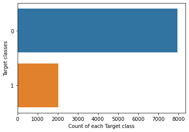
# Show the counts of observations in each categorical bin
# (column Exited) using bars.
# https://seaborn.pydata.org/generated/seaborn.countplot.html
sns.countplot(y=churn_data_encoded.Exited, data=churn_data_encoded)
plt.xlabel("Count of each Target class")
plt.ylabel("Target classes")
plt.show()

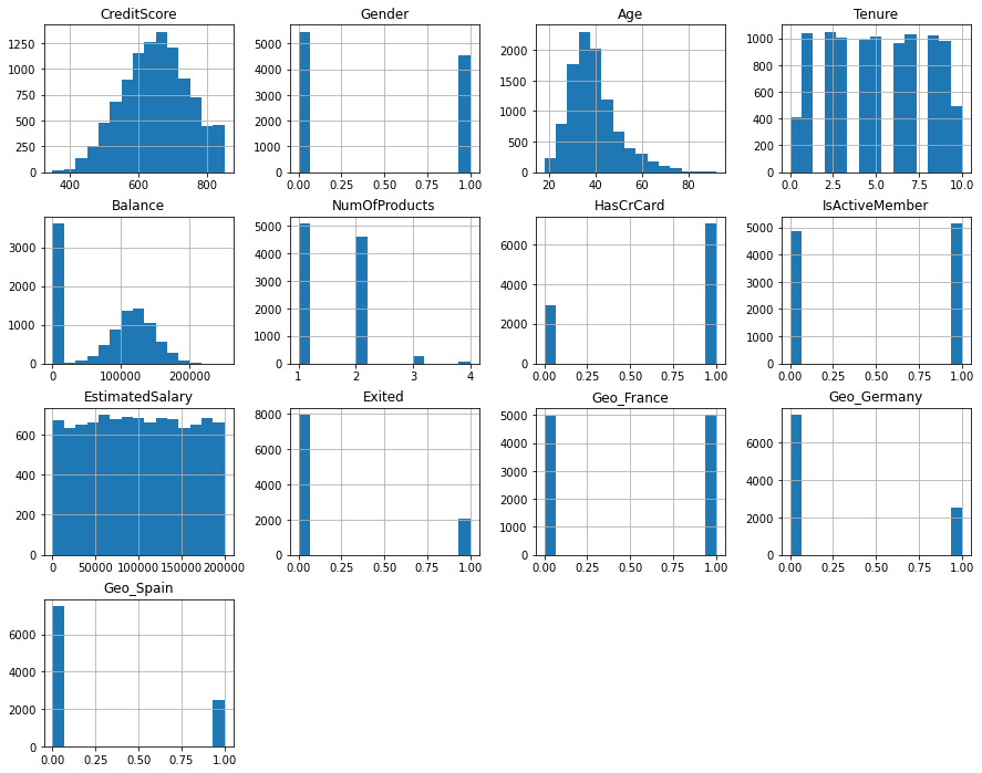
# Show distributions of the dataset
# https://pandas.pydata.org/pandas-docs/stable/reference/api/pandas.DataFrame.hist.html
# https://matplotlib.org/stable/api/_as_gen/matplotlib.pyplot.title.html
# https://matplotlib.org/stable/api/_as_gen/matplotlib.pyplot.show.html
churn_data_encoded.hist(figsize=(15, 12), bins=15)
plt.title("Features Distribution")
plt.show()

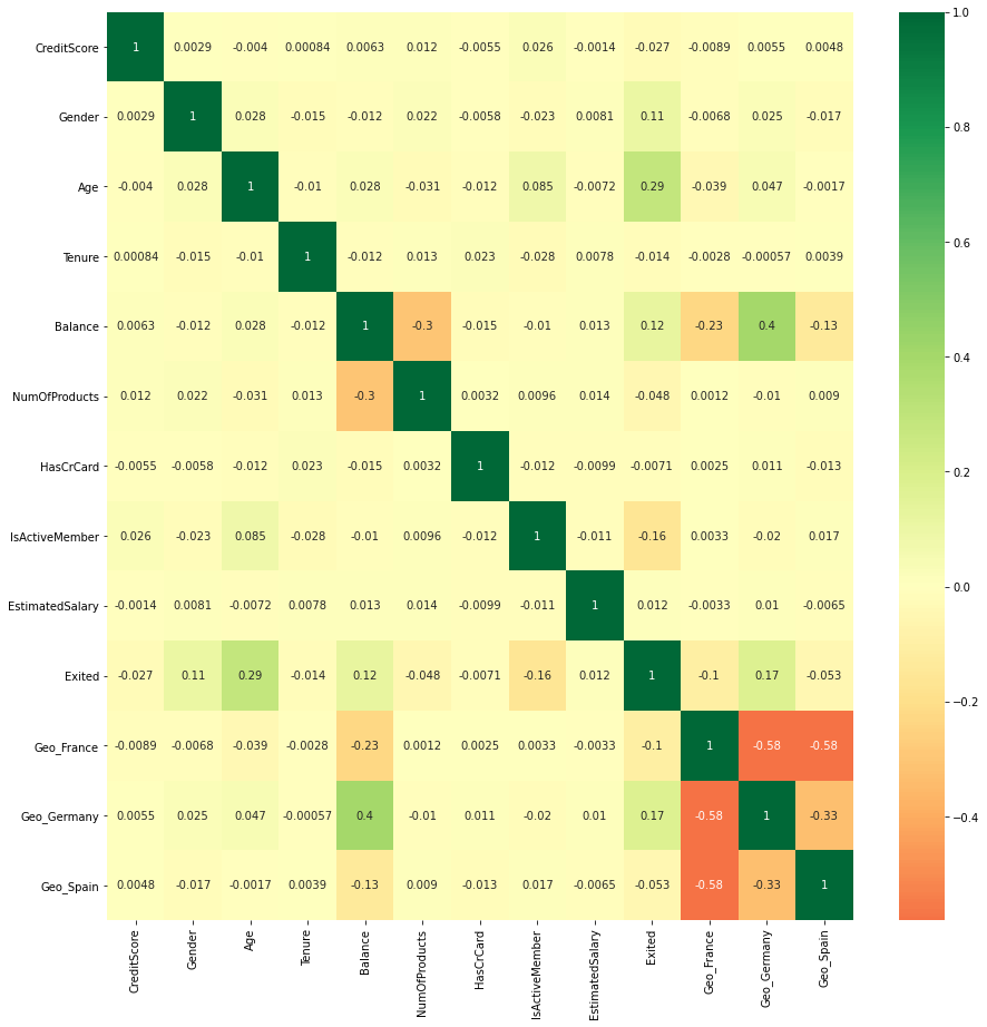
# Plot rectangular data as a color-encoded matrix.
# https://seaborn.pydata.org/generated/seaborn.heatmap.html#seaborn.heatmap
# https://matplotlib.org/stable/api/figure_api.html
plt.figure(figsize=(15, 15))
p = sns.heatmap(churn_data_encoded.corr(), annot=True, cmap="RdYlGn", center=0)

Training of the network

# Exited is target class
X = churn_data_encoded.drop(["Exited"], axis=1)
y = churn_data_encoded.Exited

# Check
X.head(10)

	CreditScore	Gender	Age	Tenure	Balance	NumOfProducts	HasCrCard	IsActiveMember	EstimatedSalary	Geo_France	Geo_Germany	Geo_Spain
RowNumber
1	619	1	42	2	0.00	1	1	1	101348.88	1	0	0
2	608	1	41	1	83807.86	1	0	1	112542.58	0	0	1
3	502	1	42	8	159660.80	3	1	0	113931.57	1	0	0
4	699	1	39	1	0.00	2	0	0	93826.63	1	0	0
5	850	1	43	2	125510.82	1	1	1	79084.10	0	0	1
6	645	0	44	8	113755.78	2	1	0	149756.71	0	0	1
7	822	0	50	7	0.00	2	1	1	10062.80	1	0	0
8	376	1	29	4	115046.74	4	1	0	119346.88	0	1	0
9	501	0	44	4	142051.07	2	0	1	74940.50	1	0	0
10	684	0	27	2	134603.88	1	1	1	71725.73	1	0	0

# Split dataset into the Training set and Test set
# https://scikit-learn.org/stable/modules/generated/sklearn.model_selection.train_test_split.html
X_train, X_test, y_train, y_test = train_test_split(
    X, y, test_size=0.33, random_state=0
)

# The dataset contains attributes with a mixtures of scales for
# various quantities.
# Many machine learning methods expect or are more effective if
# the data attributes have the same scale.
# https://machinelearningmastery.com/standardscaler-and-minmaxscaler-transforms-in-python/
# https://scikit-learn.org/stable/modules/generated/sklearn.preprocessing.StandardScaler.html
sc = StandardScaler()
X_train = sc.fit_transform(X_train)
X_test = sc.transform(X_test)

# Sequential model to initialise our ANN and dense module to build the layers.
# https://keras.io/guides/sequential_model/
# https://keras.io/api/layers/core_layers/dense/

# Create a Sequential model with 3 layers incrementally
# https://keras.io/guides/

classifier = Sequential()

# Adding the input layer and the first hidden layer
classifier.add(
    Dense(
        units=6, kernel_initializer="uniform", activation="relu", input_dim=12
    )
)
# Adding the second hidden layer
classifier.add(Dense(units=6, kernel_initializer="uniform", activation="relu"))
# Adding the output layer
classifier.add(
    Dense(units=1, kernel_initializer="uniform", activation="sigmoid")
)

# Compiling the ANN | means applying SGD on the whole ANN
classifier.compile(
    optimizer="adam", loss="binary_crossentropy", metrics=["accuracy"]
)

# Fitting the ANN to the Training set
classifier.fit(X_train, y_train, batch_size=10, epochs=100, verbose=0)

<tensorflow.python.keras.callbacks.History at 0x7f41e8445040>

Evaluations

score, acc = classifier.evaluate(X_train, y_train, batch_size=10)
print("Train score:", score)
print("Train accuracy:", acc)

# Making predictions and evaluating the model
# Predicting the Test set results
y_pred = classifier.predict(X_test)
y_pred = y_pred > 0.5

print("*" * 20)
score, acc = classifier.evaluate(X_test, y_test, batch_size=10)
print("Test score:", score)
print("Test accuracy:", acc)

# Making the Confusion Matrix
cm = confusion_matrix(y_test, y_pred)

# Evaluation metrics
p = sns.heatmap(pd.DataFrame(cm), annot=True, cmap="YlGnBu", fmt="g")
plt.title("Confusion matrix", y=1.1)
plt.ylabel("Actual label")
plt.xlabel("Predicted label")

# https://scikit-learn.org/stable/modules/generated/sklearn.metrics.roc_curve.html
y_pred = classifier.predict(X_test)
fpr, tpr, thresholds = roc_curve(y_test, y_pred)
plt.plot([0, 1], [0, 1], "k--")
plt.plot(fpr, tpr, label="ANN")
plt.xlabel("fpr")
plt.ylabel("tpr")
plt.title("ROC curve")
plt.show()

# Area under ROC curve
roc_auc_score(y_test, y_pred)