IBM stock price prediction

Predicting the next day’s stock price based on historical prices using a cleaned-up version of Apple’s historical stock data sourced from the Nasdaq website.

raise SystemExit("Stop right there!");

An exception has occurred, use %tb to see the full traceback.

SystemExit: Stop right there!

Importing libraries and packages

# System
import os

# Mathematical operations and data manipulation
import numpy as np
import pandas as pd
import math

# Modelling
from sklearn.preprocessing import MinMaxScaler
import tensorflow as tf
import keras
from tensorflow.keras import layers

# Plotting
import matplotlib.pyplot as plt
from IPython.display import display, HTML

%matplotlib inline
display(HTML("<style>.container {width:80% !important;}</style>"))

print("Tensorflow version:", tf.__version__)
print("Keras version:", keras.__version__)

Tensorflow version: 2.4.1
Keras version: 2.4.3

os.environ["TF_CPP_MIN_LOG_LEVEL"] = "2"

Set paths

# Path to datasets directory
data_path = "./datasets"
# Path to assets directory (for saving results to)
assets_path = "./assets"

Loading dataset

dataset = pd.read_csv(f"{data_path}/IBM.csv")

dataset.head()

	Date	Close	Volume	Open	High	Low
0	1/24/2020	140.56	5580189	143.39	143.9200	140.46
1	1/23/2020	142.87	5657790	144.20	144.4097	142.15
2	1/22/2020	143.89	16470430	143.32	145.7900	142.55
3	1/21/2020	139.17	7244079	137.81	139.3500	137.60
4	1/17/2020	138.31	5623336	136.54	138.3300	136.16

dataset.tail()

	Date	Close	Volume	Open	High	Low
2513	1/29/2010	122.39	11571890	124.32	125.000	121.90
2514	1/28/2010	123.75	9616132	127.03	127.040	123.05
2515	1/27/2010	126.33	8719147	125.82	126.960	125.04
2516	1/26/2010	125.75	7135190	125.92	127.750	125.41
2517	1/25/2010	126.12	5738455	126.33	126.895	125.71

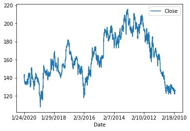
Exploring dataset

dataset.plot("Date", "Close")
plt.show()

# Reversing the data for convenience of plotting and handling
dataset = dataset.sort_index(ascending=False)

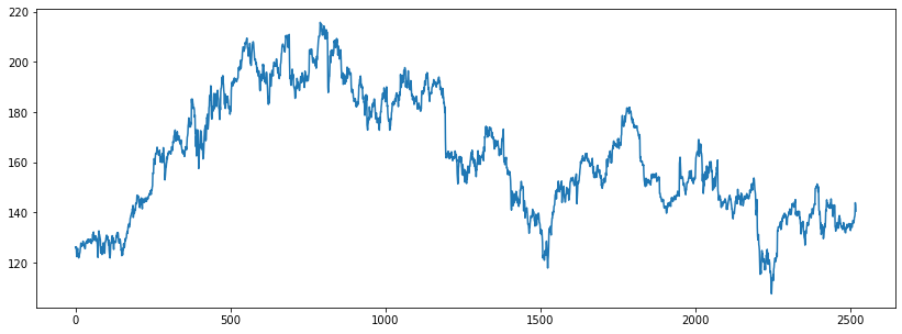
# Extracting values for ‘Close’ from the dataframe as a numpy array.
ts_data = dataset.Close.values.reshape(-1, 1)

plt.figure(figsize=(14, 5))
plt.plot(ts_data)
plt.show()

Preparing the data

# Preparing the data for stock price prediction
train_recs = int(len(ts_data) * 0.75)

train_data = ts_data[:train_recs]
test_data = ts_data[train_recs:]

len(train_data), len(test_data)

(1888, 630)

# Scaling
scaler = MinMaxScaler()
train_scaled = scaler.fit_transform(train_data)
test_scaled = scaler.transform(test_data)

def get_lookback(inp, look_back):
    y = pd.DataFrame(inp)
    dataX = [y.shift(i) for i in range(1, look_back + 1)]
    dataX = pd.concat(dataX, axis=1)
    dataX.fillna(0, inplace=True)
    return dataX.values, y.values

look_back = 10
trainX, trainY = get_lookback(train_scaled, look_back=look_back)
testX, testY = get_lookback(test_scaled, look_back=look_back)

trainX.shape, testX.shape

((1888, 10), (630, 10))

Hybrid model

# Training a hybrid (1D conv + RNN) model, with a
model_hybrid = tf.keras.Sequential(
    [
        layers.Reshape((look_back, 1), input_shape=(look_back,)),
        layers.Conv1D(5, 3, activation="relu"),
        layers.SimpleRNN(32),
        layers.Dropout(0.25),
        layers.Dense(1),
        layers.Activation("linear"),
    ]
)

model_hybrid.compile(loss="mean_squared_error", optimizer="adam")

model_hybrid.summary()

Model: "sequential"
_________________________________________________________________
Layer (type)                 Output Shape              Param #   
=================================================================
reshape (Reshape)            (None, 10, 1)             0         
_________________________________________________________________
conv1d (Conv1D)              (None, 8, 5)              20        
_________________________________________________________________
simple_rnn (SimpleRNN)       (None, 32)                1216      
_________________________________________________________________
dropout (Dropout)            (None, 32)                0         
_________________________________________________________________
dense (Dense)                (None, 1)                 33        
_________________________________________________________________
activation (Activation)      (None, 1)                 0         
=================================================================
Total params: 1,269
Trainable params: 1,269
Non-trainable params: 0
_________________________________________________________________

model_hybrid.fit(
    trainX, trainY, epochs=3, batch_size=1, verbose=2, validation_split=0.1
)

Epoch 1/3
1699/1699 - 18s - loss: 0.0089 - val_loss: 0.0012
Epoch 2/3
1699/1699 - 20s - loss: 0.0049 - val_loss: 9.7144e-04
Epoch 3/3
1699/1699 - 18s - loss: 0.0037 - val_loss: 7.5165e-04

<tensorflow.python.keras.callbacks.History at 0x7f4c82a63970>

def calculate_performance(model_obj):

    score_train = model_obj.evaluate(trainX, trainY, verbose=0)
    print("Train RMSE: %.2f RMSE" % (math.sqrt(score_train)))

    score_test = model_obj.evaluate(testX, testY, verbose=0)
    print("Test RMSE: %.2f RMSE" % (math.sqrt(score_test)))


calculate_performance(model_hybrid)

Train RMSE: 0.03 RMSE
Test RMSE: 0.04 RMSE

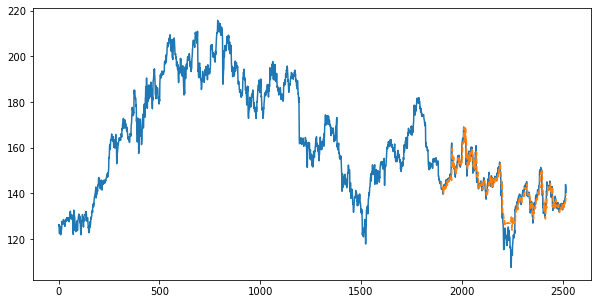
def plot_prediction(model_obj):
    testPredict = scaler.inverse_transform(model_obj.predict(testX))

    pred_test_plot = ts_data.copy()
    pred_test_plot[: train_recs + look_back, :] = np.nan
    pred_test_plot[train_recs + look_back :, :] = testPredict[look_back:]

    plt.plot(ts_data)
    plt.plot(pred_test_plot, "--")


plt.figure(figsize=(10, 5))
plot_prediction(model_hybrid)