EDA Ames housing set

Analysis:

1. The target variable

2. Variable types (categorical and numerical)

3. Missing data

4. Numerical variables

   • Discrete

   • Continuous

   • Distributions

   • Transformations

5. Categorical variables

   • Cardinality

   • Rare Labels

   • Special mappings

6. Additional Reading Resources

Imports and packages

# to handle datasets
import pandas as pd
import numpy as np

# for plotting
import matplotlib.pyplot as plt
import seaborn as sns

# for the yeo-johnson transformation
import scipy.stats as stats

# to display all the columns of the dataframe in the notebook
pd.pandas.set_option("display.max_columns", None)

Paths

# Path to datasets directory
data_path = "./datasets"
# Path to assets directory (for saving results to)
assets_path = "./assets"

Prepare the data set

# load dataset
data = pd.read_csv(f"{data_path}/train.csv")

# rows and columns of the data
print(data.shape)

# visualise the dataset
data.head()

(1460, 81)

	Id	MSSubClass	MSZoning	LotFrontage	LotArea	Street	Alley	LotShape	LandContour	Utilities	LotConfig	LandSlope	Neighborhood	Condition1	Condition2	BldgType	HouseStyle	OverallQual	OverallCond	YearBuilt	YearRemodAdd	RoofStyle	RoofMatl	Exterior1st	Exterior2nd	MasVnrType	MasVnrArea	ExterQual	ExterCond	Foundation	BsmtQual	BsmtCond	BsmtExposure	BsmtFinType1	BsmtFinSF1	BsmtFinType2	BsmtFinSF2	BsmtUnfSF	TotalBsmtSF	Heating	HeatingQC	CentralAir	Electrical	1stFlrSF	2ndFlrSF	LowQualFinSF	GrLivArea	BsmtFullBath	BsmtHalfBath	FullBath	HalfBath	BedroomAbvGr	KitchenAbvGr	KitchenQual	TotRmsAbvGrd	Functional	Fireplaces	FireplaceQu	GarageType	GarageYrBlt	GarageFinish	GarageCars	GarageArea	GarageQual	GarageCond	PavedDrive	WoodDeckSF	OpenPorchSF	EnclosedPorch	3SsnPorch	ScreenPorch	PoolArea	PoolQC	Fence	MiscFeature	MiscVal	MoSold	YrSold	SaleType	SaleCondition	SalePrice
0	1	60	RL	65.0	8450	Pave	NaN	Reg	Lvl	AllPub	Inside	Gtl	CollgCr	Norm	Norm	1Fam	2Story	7	5	2003	2003	Gable	CompShg	VinylSd	VinylSd	BrkFace	196.0	Gd	TA	PConc	Gd	TA	No	GLQ	706	Unf	0	150	856	GasA	Ex	Y	SBrkr	856	854	0	1710	1	0	2	1	3	1	Gd	8	Typ	0	NaN	Attchd	2003.0	RFn	2	548	TA	TA	Y	0	61	0	0	0	0	NaN	NaN	NaN	0	2	2008	WD	Normal	208500
1	2	20	RL	80.0	9600	Pave	NaN	Reg	Lvl	AllPub	FR2	Gtl	Veenker	Feedr	Norm	1Fam	1Story	6	8	1976	1976	Gable	CompShg	MetalSd	MetalSd	None	0.0	TA	TA	CBlock	Gd	TA	Gd	ALQ	978	Unf	0	284	1262	GasA	Ex	Y	SBrkr	1262	0	0	1262	0	1	2	0	3	1	TA	6	Typ	1	TA	Attchd	1976.0	RFn	2	460	TA	TA	Y	298	0	0	0	0	0	NaN	NaN	NaN	0	5	2007	WD	Normal	181500
2	3	60	RL	68.0	11250	Pave	NaN	IR1	Lvl	AllPub	Inside	Gtl	CollgCr	Norm	Norm	1Fam	2Story	7	5	2001	2002	Gable	CompShg	VinylSd	VinylSd	BrkFace	162.0	Gd	TA	PConc	Gd	TA	Mn	GLQ	486	Unf	0	434	920	GasA	Ex	Y	SBrkr	920	866	0	1786	1	0	2	1	3	1	Gd	6	Typ	1	TA	Attchd	2001.0	RFn	2	608	TA	TA	Y	0	42	0	0	0	0	NaN	NaN	NaN	0	9	2008	WD	Normal	223500
3	4	70	RL	60.0	9550	Pave	NaN	IR1	Lvl	AllPub	Corner	Gtl	Crawfor	Norm	Norm	1Fam	2Story	7	5	1915	1970	Gable	CompShg	Wd Sdng	Wd Shng	None	0.0	TA	TA	BrkTil	TA	Gd	No	ALQ	216	Unf	0	540	756	GasA	Gd	Y	SBrkr	961	756	0	1717	1	0	1	0	3	1	Gd	7	Typ	1	Gd	Detchd	1998.0	Unf	3	642	TA	TA	Y	0	35	272	0	0	0	NaN	NaN	NaN	0	2	2006	WD	Abnorml	140000
4	5	60	RL	84.0	14260	Pave	NaN	IR1	Lvl	AllPub	FR2	Gtl	NoRidge	Norm	Norm	1Fam	2Story	8	5	2000	2000	Gable	CompShg	VinylSd	VinylSd	BrkFace	350.0	Gd	TA	PConc	Gd	TA	Av	GLQ	655	Unf	0	490	1145	GasA	Ex	Y	SBrkr	1145	1053	0	2198	1	0	2	1	4	1	Gd	9	Typ	1	TA	Attchd	2000.0	RFn	3	836	TA	TA	Y	192	84	0	0	0	0	NaN	NaN	NaN	0	12	2008	WD	Normal	250000

# drop id, it is just a number given to identify each house
data.drop("Id", axis=1, inplace=True)

data.shape

(1460, 80)

The house price dataset contains 1460 rows, that is, houses, and 80 columns, i.e., variables.

79 are predictive variables and 1 is the target variable: SalePrice

Target

# histogran to evaluate target distribution

data["SalePrice"].hist(bins=50, density=True)
plt.ylabel("Number of houses")
plt.xlabel("Sale Price")
plt.show()

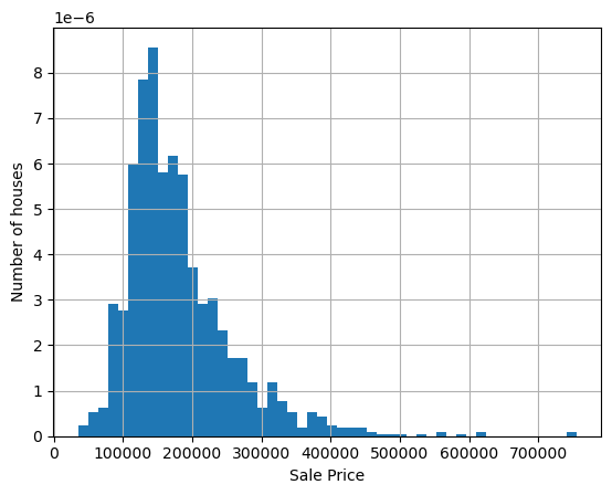
The target is continuous, and the distribution is skewed towards the right.

The value spread can be improved with a mathematical transformation.

# Transforming the target using logarithm

np.log(data["SalePrice"]).hist(bins=50, density=True)
plt.ylabel("Number of houses")
plt.xlabel("Log of Sale Price")
plt.show()

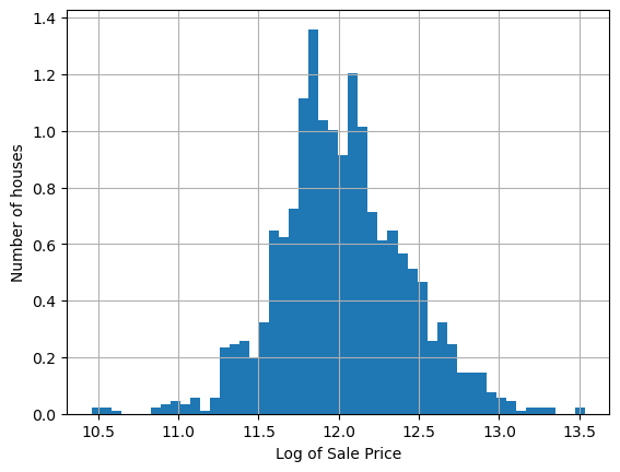
Now the distribution looks more Gaussian.

Variable Types

# Identifying the categorical variables, capturing those of type *object*

cat_vars = [var for var in data.columns if data[var].dtype == "O"]

# MSSubClass is also categorical by definition, despite its numeric values
# (you can find the definitions of the variables in the data_description.txt
# file available on Kaggle, in the same website where you downloaded the data)

# Adding MSSubClass to the list of categorical variables
cat_vars = cat_vars + ["MSSubClass"]

# Number of categorical variables
len(cat_vars)

44

# Casting categorical variables
data[cat_vars] = data[cat_vars].astype("O")

# Identifying numerical variables
num_vars = [
    var for var in data.columns if var not in cat_vars and var != "SalePrice"
]

# Number of numerical variables
len(num_vars)

35

Missing values

# List of the variables that contain missing values
vars_with_na = [var for var in data.columns if data[var].isnull().sum() > 0]

# Percentage of missing values (expressed as decimals)
# and displaying the result ordered by % of missing data

data[vars_with_na].isnull().mean().sort_values(ascending=False)

PoolQC          0.995205
MiscFeature     0.963014
Alley           0.937671
Fence           0.807534
FireplaceQu     0.472603
LotFrontage     0.177397
GarageType      0.055479
GarageYrBlt     0.055479
GarageFinish    0.055479
GarageQual      0.055479
GarageCond      0.055479
BsmtExposure    0.026027
BsmtFinType2    0.026027
BsmtFinType1    0.025342
BsmtCond        0.025342
BsmtQual        0.025342
MasVnrArea      0.005479
MasVnrType      0.005479
Electrical      0.000685
dtype: float64

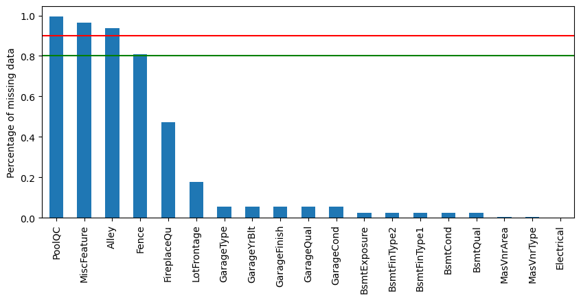
The dataset contains a few variables with a big proportion of missing values (4 variables at the top). And some other variables with a small percentage of missing observations.

This means that to train a machine learning model with this data set, the missing data in these variables must be imputed.

Visualizing the percentage of missing values in the variables:

# Plotting
data[vars_with_na].isnull().mean().sort_values(ascending=False).plot.bar(
    figsize=(10, 4)
)
plt.ylabel("Percentage of missing data")
plt.axhline(y=0.90, color="r", linestyle="-")
plt.axhline(y=0.80, color="g", linestyle="-")

plt.show()

# Determining which variables, from those with missing data,
# are numerical and which are categorical
cat_na = [var for var in cat_vars if var in vars_with_na]
num_na = [var for var in num_vars if var in vars_with_na]

print("Number of categorical variables with na: ", len(cat_na))
print("Number of numerical variables with na: ", len(num_na))

Number of categorical variables with na:  16
Number of numerical variables with na:  3

num_na

['LotFrontage', 'MasVnrArea', 'GarageYrBlt']

cat_na

['Alley',
 'MasVnrType',
 'BsmtQual',
 'BsmtCond',
 'BsmtExposure',
 'BsmtFinType1',
 'BsmtFinType2',
 'Electrical',
 'FireplaceQu',
 'GarageType',
 'GarageFinish',
 'GarageQual',
 'GarageCond',
 'PoolQC',
 'Fence',
 'MiscFeature']

Relationship between missing data and Sale Price

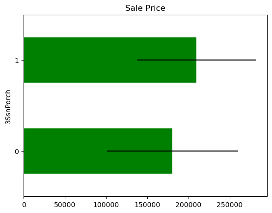
The price of the house in those observations where the information is missing,for each variable that shows missing data.

def analyse_na_value(df, var):

    # copy of the dataframe, so as not to override the original data
    # see the link for more details about pandas.copy()
    # https://pandas.pydata.org/pandas-docs/stable/reference/api/pandas.DataFrame.copy.html
    df = df.copy()

    # making an interim variable that indicates 1 if the
    # observation was missing or 0 otherwise
    df[var] = np.where(df[var].isnull(), 1, 0)

    # comparing the median SalePrice in the observations where data is missing
    # vs the observations where data is available

    # determining the median price in the groups 1 and 0,
    # and the standard deviation of the sale price,
    # and capturing the results in a temporary dataset
    temp = df.groupby(var)["SalePrice"].agg(["mean", "std"])

    # plotting into a bar graph
    temp.plot(
        kind="barh",
        y="mean",
        legend=False,
        xerr="std",
        title="Sale Price",
        color="green",
    )

    plt.show()

# Running the function on each variable with missing data
for var in vars_with_na:
    analyse_na_value(data, var)

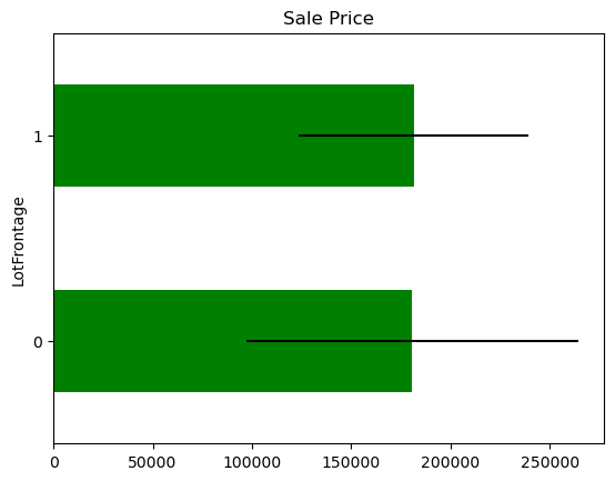
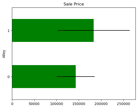
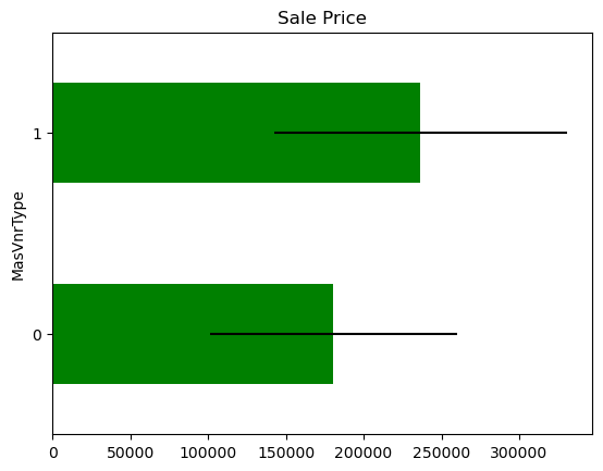
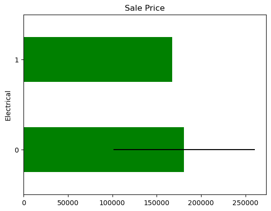
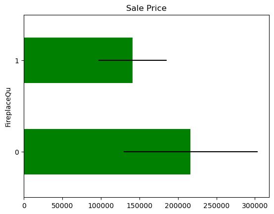
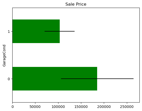
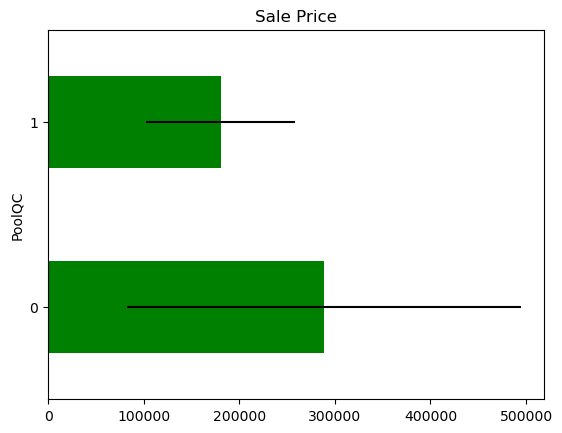
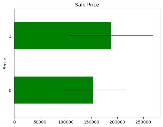
In some variables, the average Sale Price in houses where the information is missing, differs from the average Sale Price in houses where information exists. This suggests that data being missing could be a good predictor of Sale Price.

Numerical variables

print("Number of numerical variables: ", len(num_vars))

# Visualizing the numerical variables
data[num_vars].head()

Number of numerical variables:  35

	LotFrontage	LotArea	OverallQual	OverallCond	YearBuilt	YearRemodAdd	MasVnrArea	BsmtFinSF1	BsmtFinSF2	BsmtUnfSF	TotalBsmtSF	1stFlrSF	2ndFlrSF	LowQualFinSF	GrLivArea	BsmtFullBath	BsmtHalfBath	FullBath	HalfBath	BedroomAbvGr	KitchenAbvGr	TotRmsAbvGrd	Fireplaces	GarageYrBlt	GarageCars	GarageArea	WoodDeckSF	OpenPorchSF	EnclosedPorch	3SsnPorch	ScreenPorch	PoolArea	MiscVal	MoSold	YrSold
0	65.0	8450	7	5	2003	2003	196.0	706	0	150	856	856	854	0	1710	1	0	2	1	3	1	8	0	2003.0	2	548	0	61	0	0	0	0	0	2	2008
1	80.0	9600	6	8	1976	1976	0.0	978	0	284	1262	1262	0	0	1262	0	1	2	0	3	1	6	1	1976.0	2	460	298	0	0	0	0	0	0	5	2007
2	68.0	11250	7	5	2001	2002	162.0	486	0	434	920	920	866	0	1786	1	0	2	1	3	1	6	1	2001.0	2	608	0	42	0	0	0	0	0	9	2008
3	60.0	9550	7	5	1915	1970	0.0	216	0	540	756	961	756	0	1717	1	0	1	0	3	1	7	1	1998.0	3	642	0	35	272	0	0	0	0	2	2006
4	84.0	14260	8	5	2000	2000	350.0	655	0	490	1145	1145	1053	0	2198	1	0	2	1	4	1	9	1	2000.0	3	836	192	84	0	0	0	0	0	12	2008

Temporal variables

There are 4 year variables in the dataset:

• YearBuilt: year in which the house was built

• YearRemodAdd: year in which the house was remodeled

• GarageYrBlt: year in which a garage was built

• YrSold: year in which the house was sold

Extracting information from date variables in their raw format: For example, capturing the difference in years between the year the house was built and the year the house was sold.

# List of variables that contain year information

year_vars = [var for var in num_vars if "Yr" in var or "Year" in var]

year_vars

['YearBuilt', 'YearRemodAdd', 'GarageYrBlt', 'YrSold']

# Exploring the values of these temporal variables
for var in year_vars:
    print(var, data[var].unique())
    print()

YearBuilt [2003 1976 2001 1915 2000 1993 2004 1973 1931 1939 1965 2005 1962 2006
 1960 1929 1970 1967 1958 1930 2002 1968 2007 1951 1957 1927 1920 1966
 1959 1994 1954 1953 1955 1983 1975 1997 1934 1963 1981 1964 1999 1972
 1921 1945 1982 1998 1956 1948 1910 1995 1991 2009 1950 1961 1977 1985
 1979 1885 1919 1990 1969 1935 1988 1971 1952 1936 1923 1924 1984 1926
 1940 1941 1987 1986 2008 1908 1892 1916 1932 1918 1912 1947 1925 1900
 1980 1989 1992 1949 1880 1928 1978 1922 1996 2010 1946 1913 1937 1942
 1938 1974 1893 1914 1906 1890 1898 1904 1882 1875 1911 1917 1872 1905]

YearRemodAdd [2003 1976 2002 1970 2000 1995 2005 1973 1950 1965 2006 1962 2007 1960
 2001 1967 2004 2008 1997 1959 1990 1955 1983 1980 1966 1963 1987 1964
 1972 1996 1998 1989 1953 1956 1968 1981 1992 2009 1982 1961 1993 1999
 1985 1979 1977 1969 1958 1991 1971 1952 1975 2010 1984 1986 1994 1988
 1954 1957 1951 1978 1974]

GarageYrBlt [2003. 1976. 2001. 1998. 2000. 1993. 2004. 1973. 1931. 1939. 1965. 2005.
 1962. 2006. 1960. 1991. 1970. 1967. 1958. 1930. 2002. 1968. 2007. 2008.
 1957. 1920. 1966. 1959. 1995. 1954. 1953.   nan 1983. 1977. 1997. 1985.
 1963. 1981. 1964. 1999. 1935. 1990. 1945. 1987. 1989. 1915. 1956. 1948.
 1974. 2009. 1950. 1961. 1921. 1900. 1979. 1951. 1969. 1936. 1975. 1971.
 1923. 1984. 1926. 1955. 1986. 1988. 1916. 1932. 1972. 1918. 1980. 1924.
 1996. 1940. 1949. 1994. 1910. 1978. 1982. 1992. 1925. 1941. 2010. 1927.
 1947. 1937. 1942. 1938. 1952. 1928. 1922. 1934. 1906. 1914. 1946. 1908.
 1929. 1933.]

YrSold [2008 2007 2006 2009 2010]

As expected, the values are years.

Exploring the evolution of the sale price with the years in which the house was sold:

# plotting median sale price vs year in which it was sold
data.groupby("YrSold")["SalePrice"].median().plot()
plt.ylabel("Median House Price")

Text(0, 0.5, 'Median House Price')

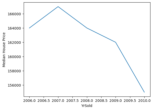
There has been a drop in the value of the houses. That is unusual, in real life, house prices typically go up as years go by.

Plotting the price of sale vs year in which it was built

# plotting median sale price vs year in which it was built

data.groupby("YearBuilt")["SalePrice"].median().plot()
plt.ylabel("Median House Price")

Text(0, 0.5, 'Median House Price')

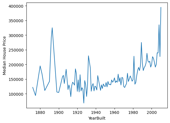
Newly built / younger houses tend to be more expensive.

Could it be that lately older houses were sold?

Capture the elapsed years between the Year variables and the year in which the house was sold:

def analyse_year_vars(df, var):

    df = df.copy()

    # capturing difference between a year variable and year
    # in which the house was sold
    df[var] = df["YrSold"] - df[var]

    df.groupby("YrSold")[var].median().plot()
    plt.ylabel("Time from " + var)
    plt.show()


for var in year_vars:
    if var != "YrSold":
        analyse_year_vars(data, var)

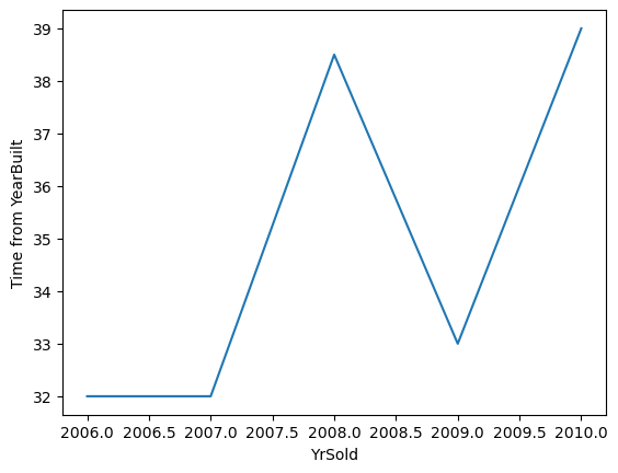
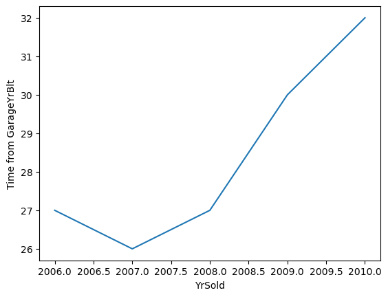
Towards 2010, the houses sold had older garages, and had not been remodelled recently, that might explain why we see cheaper sales prices in recent years, at least in this dataset.

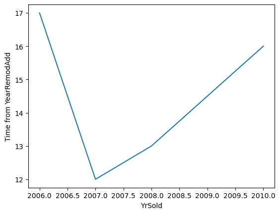
Plotting instead the time since last remodelled, or time since built, and sale price, to see if there is a relationship.

def analyse_year_vars(df, var):

    df = df.copy()

    # capturing difference between a year variable and year
    # in which the house was sold
    df[var] = df["YrSold"] - df[var]

    plt.scatter(df[var], df["SalePrice"])
    plt.ylabel("SalePrice")
    plt.xlabel(var)
    plt.show()


for var in year_vars:
    if var != "YrSold":
        analyse_year_vars(data, var)

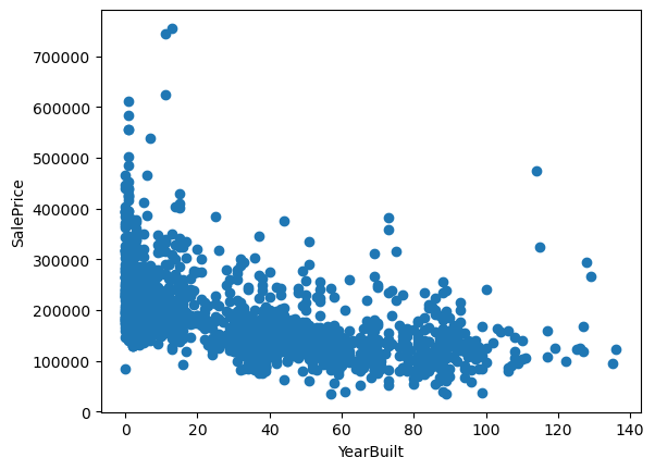
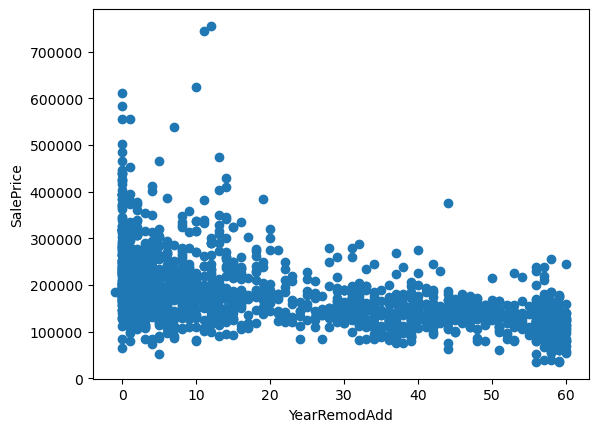
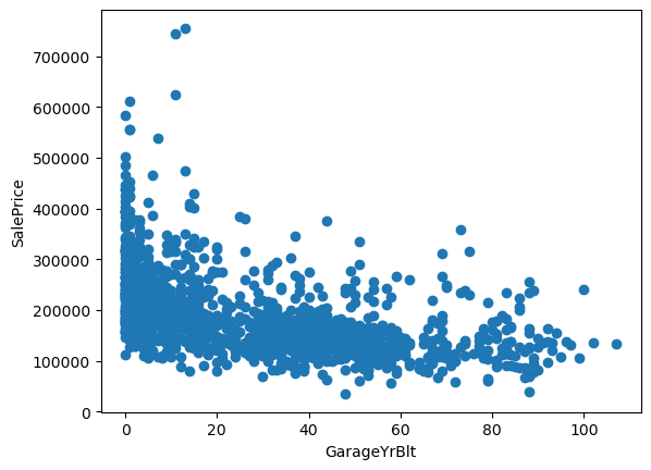
There seems to be a tendency to a decrease in price, with older houses. In other words, the longer the time between the house was built or remodeled and sale date, the lower the sale Price.

Which makes sense, cause this means that the house will have an older look, and potentially needs repairs.

Discrete variables

#  List of discrete variables
discrete_vars = [
    var
    for var in num_vars
    if len(data[var].unique()) < 20 and var not in year_vars
]

print("Number of discrete variables: ", len(discrete_vars))

Number of discrete variables:  13

# Visualise the discrete variables

data[discrete_vars].head()

	OverallQual	OverallCond	BsmtFullBath	BsmtHalfBath	FullBath	HalfBath	BedroomAbvGr	KitchenAbvGr	TotRmsAbvGrd	Fireplaces	GarageCars	PoolArea	MoSold
0	7	5	1	0	2	1	3	1	8	0	2	0	2
1	6	8	0	1	2	0	3	1	6	1	2	0	5
2	7	5	1	0	2	1	3	1	6	1	2	0	9
3	7	5	1	0	1	0	3	1	7	1	3	0	2
4	8	5	1	0	2	1	4	1	9	1	3	0	12

These discrete variables tend to be qualifications (Qual) or grading scales (Cond), or refer to the number of rooms, or units (FullBath, GarageCars), or indicate the area of the room (KitchenAbvGr).

We expect higher prices, with bigger numbers. Analysing their contribution to the house price.

MoSold is the month in which the house was sold.

for var in discrete_vars:
    # make boxplot with Catplot
    sns.catplot(
        x=var, y="SalePrice", data=data, kind="box", height=4, aspect=1.5
    )
    # add data points to boxplot with stripplot
    sns.stripplot(
        x=var, y="SalePrice", data=data, jitter=0.1, alpha=0.3, color="k"
    )
    plt.show()

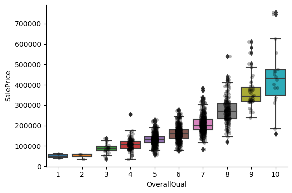
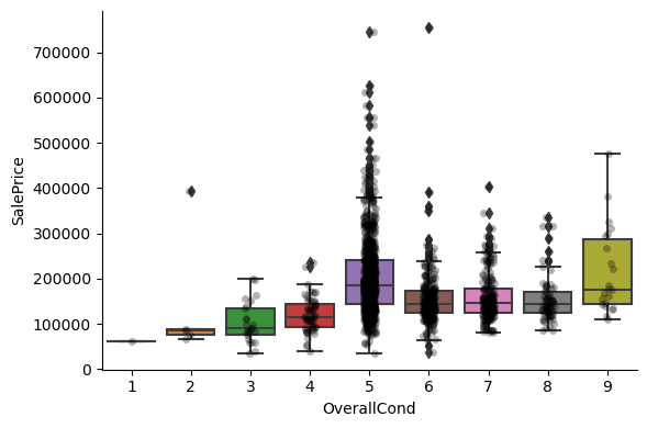
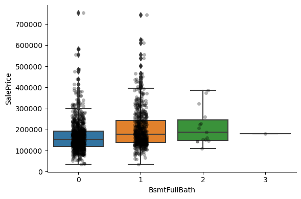
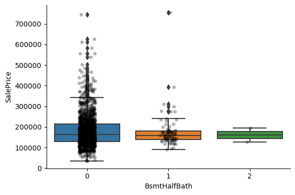
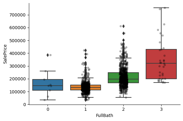
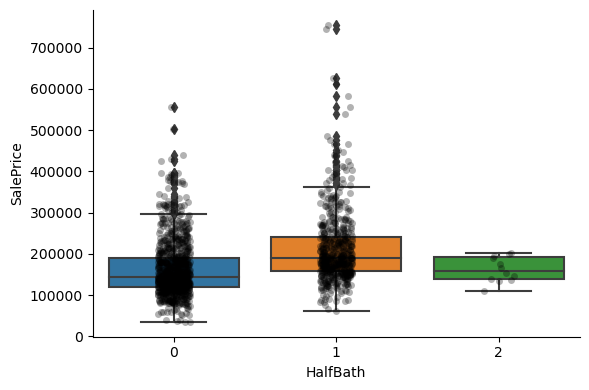
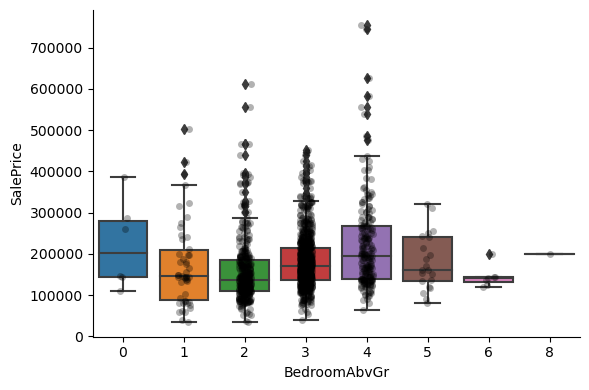
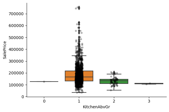
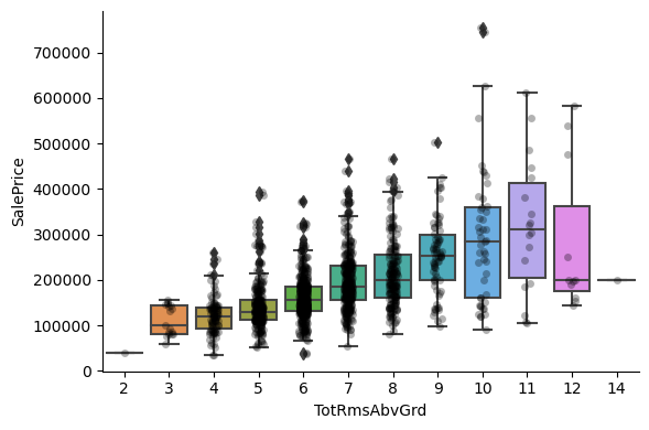
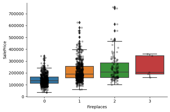
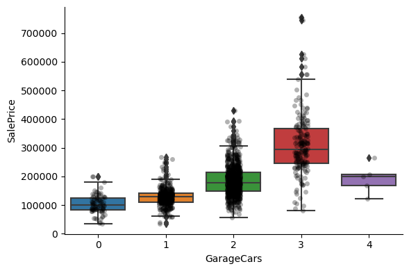
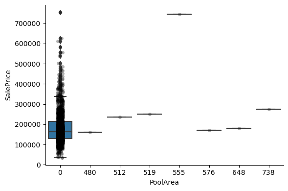
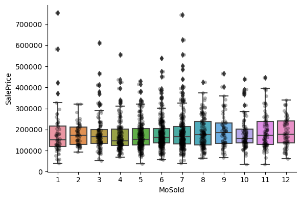
For most discrete numerical variables, the sale price increases with the quality, or overall condition, or number of rooms, or surface.

For some variables, this tendency can not be seen. Most likely that variable is not a good predictor of sale price.

Continuous variables

Distribution of the continuous variables.

# List of continuous variables
cont_vars = [var for var in num_vars if var not in discrete_vars + year_vars]

print("Number of continuous variables: ", len(cont_vars))

Number of continuous variables:  18

# Visualising the continuous variables

data[cont_vars].head()

	LotFrontage	LotArea	MasVnrArea	BsmtFinSF1	BsmtFinSF2	BsmtUnfSF	TotalBsmtSF	1stFlrSF	2ndFlrSF	LowQualFinSF	GrLivArea	GarageArea	WoodDeckSF	OpenPorchSF	EnclosedPorch	3SsnPorch	ScreenPorch	MiscVal
0	65.0	8450	196.0	706	0	150	856	856	854	0	1710	548	0	61	0	0	0	0
1	80.0	9600	0.0	978	0	284	1262	1262	0	0	1262	460	298	0	0	0	0	0
2	68.0	11250	162.0	486	0	434	920	920	866	0	1786	608	0	42	0	0	0	0
3	60.0	9550	0.0	216	0	540	756	961	756	0	1717	642	0	35	272	0	0	0
4	84.0	14260	350.0	655	0	490	1145	1145	1053	0	2198	836	192	84	0	0	0	0

# Plotting histograms for all continuous variables

data[cont_vars].hist(bins=30, figsize=(15, 15))
plt.show()

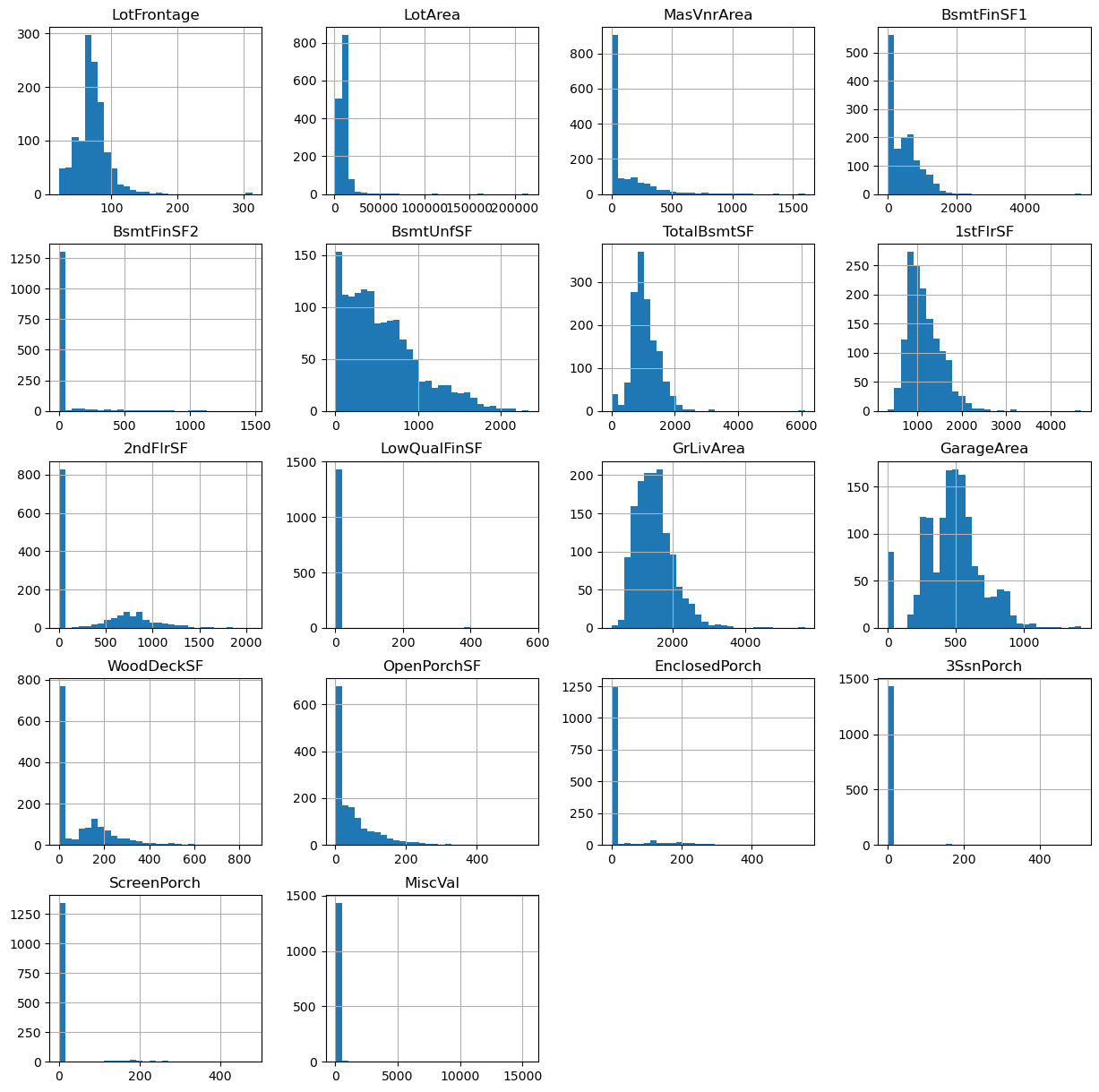
The variables are not normally distributed. And there are a particular few that are extremely skewed like 3SsnPorch, ScreenPorch and MiscVal.

Sometimes, transforming the variables to improve the value spread, improves the model performance. But it is unlikely that a transformation will help change the distribution of the super skewed variables dramatically.

Applying a Yeo-Johnson transformation to variables like LotFrontage, LotArea, BsmUnfSF, and a binary transformation to variables like 3SsnPorch, ScreenPorch and MiscVal.

# List with the super skewed variables for later

skewed = [
    "BsmtFinSF2",
    "LowQualFinSF",
    "EnclosedPorch",
    "3SsnPorch",
    "ScreenPorch",
    "MiscVal",
]

# Capturing the remaining continuous variables

cont_vars = [
    "LotFrontage",
    "LotArea",
    "MasVnrArea",
    "BsmtFinSF1",
    "BsmtUnfSF",
    "TotalBsmtSF",
    "1stFlrSF",
    "2ndFlrSF",
    "GrLivArea",
    "GarageArea",
    "WoodDeckSF",
    "OpenPorchSF",
]

Yeo-Johnson transformation

# Analysing the distributions of the variables
# after applying a yeo-johnson transformation

# temporary copy of the data
tmp = data.copy()

for var in cont_vars:

    # transform the variable - yeo-johsnon
    tmp[var], param = stats.yeojohnson(data[var])


# plot the histograms of the transformed variables
tmp[cont_vars].hist(bins=30, figsize=(15, 15))
plt.show()

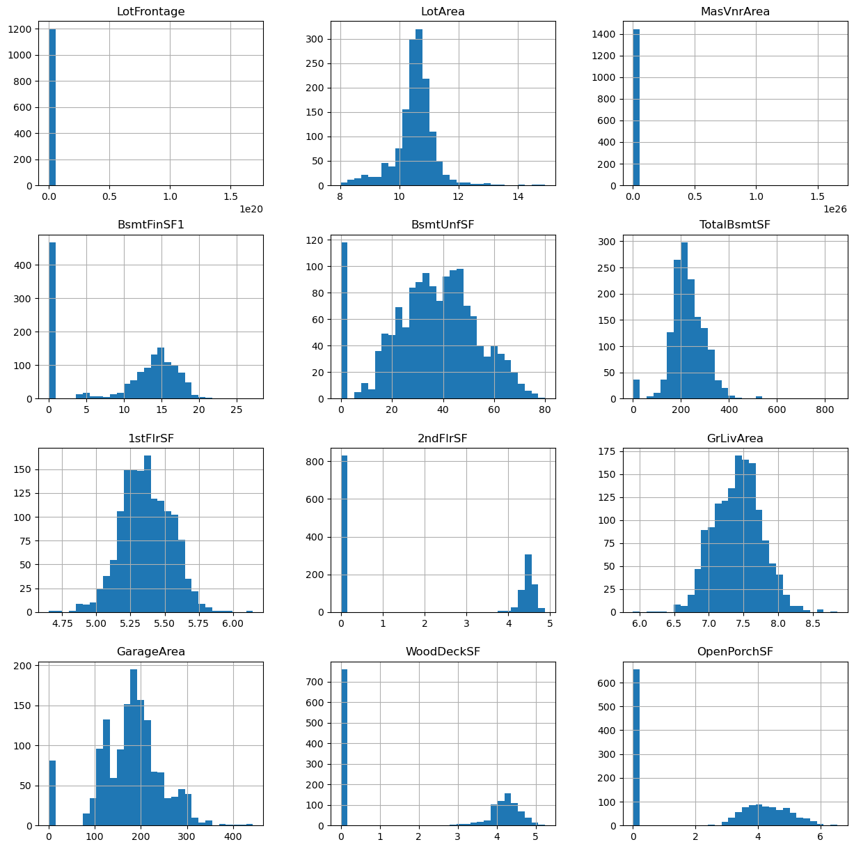
For LotFrontage and MasVnrArea the transformation did not do an amazing job.

For the others, the values seem to be spread more evenly in the range.

Whether this helps improve the predictive power, remains to be seen. To determine if this is the case, train a model with the original values and one with the transformed values, and determine model performance, and feature importance.

Here, we do a quick visual exploration instead:

# Plotting the original or transformed variables
# vs sale price, and see if there is a relationship

for var in cont_vars:

    plt.figure(figsize=(12, 4))

    # plot the original variable vs sale price
    plt.subplot(1, 2, 1)
    plt.scatter(data[var], np.log(data["SalePrice"]))
    plt.ylabel("Sale Price")
    plt.xlabel("Original " + var)

    # plot transformed variable vs sale price
    plt.subplot(1, 2, 2)
    plt.scatter(tmp[var], np.log(tmp["SalePrice"]))
    plt.ylabel("Sale Price")
    plt.xlabel("Transformed " + var)

    plt.show()

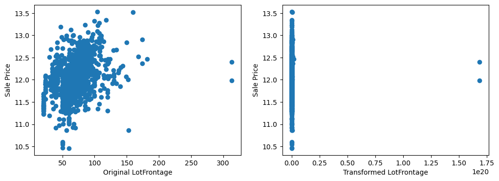
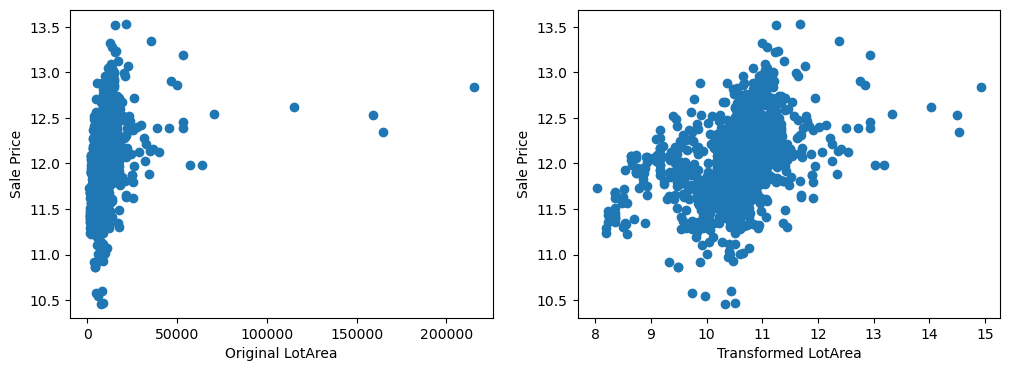
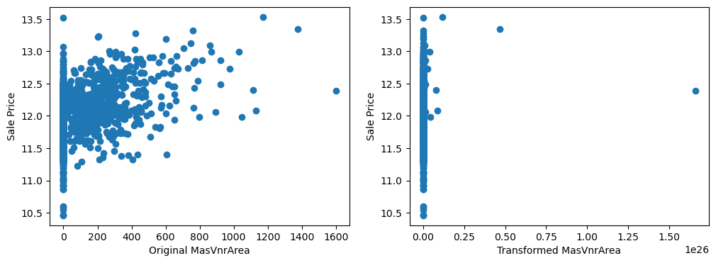
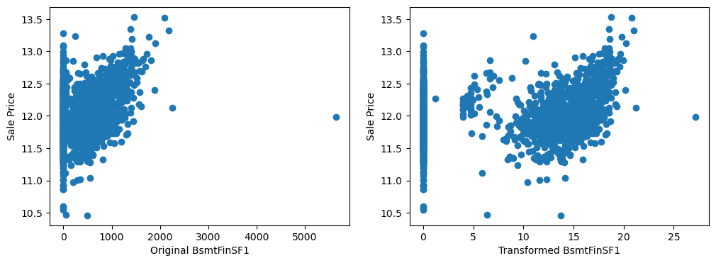
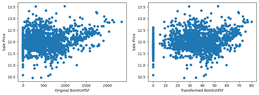
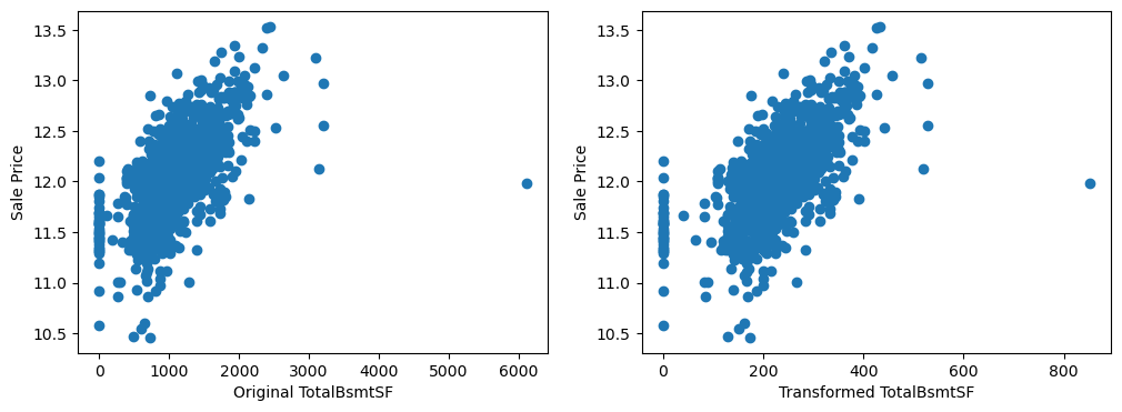
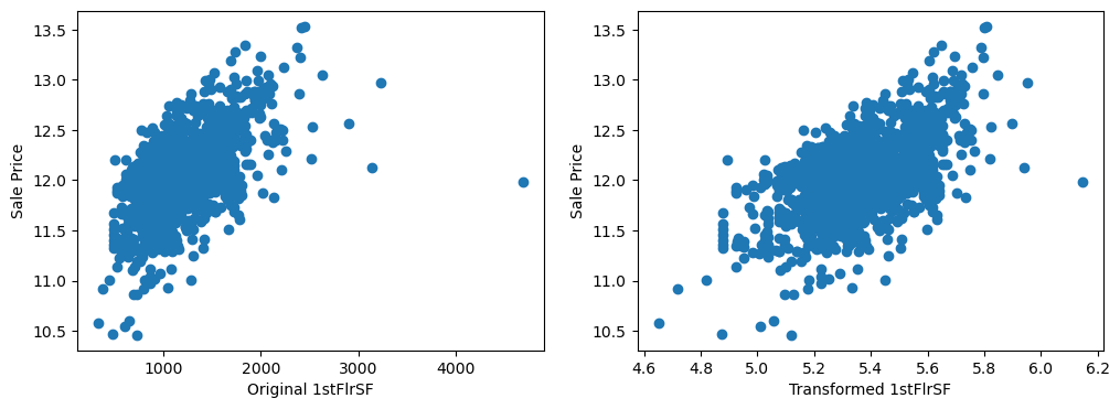
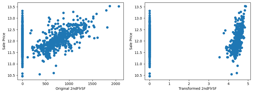
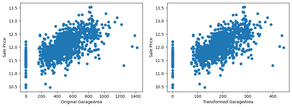
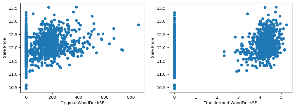
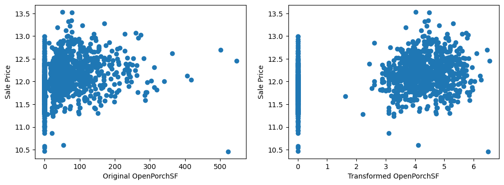
By eye, the transformations seems to improve the relationship only for LotArea.

A different transformation: Most variables contain the value 0, and thus the logarithmic transformation can not be applied, but it can be applied for the following variables:

[“LotFrontage”, “1stFlrSF”, “GrLivArea”]

Check if that changes the variable distribution and its relationship with the target.

Logarithmic transformation

# Analysing the distributions of these variables
# after applying a logarithmic transformation

tmp = data.copy()

for var in ["LotFrontage", "1stFlrSF", "GrLivArea"]:

    # transform the variable with logarithm
    tmp[var] = np.log(data[var])

tmp[["LotFrontage", "1stFlrSF", "GrLivArea"]].hist(bins=30)
plt.show()

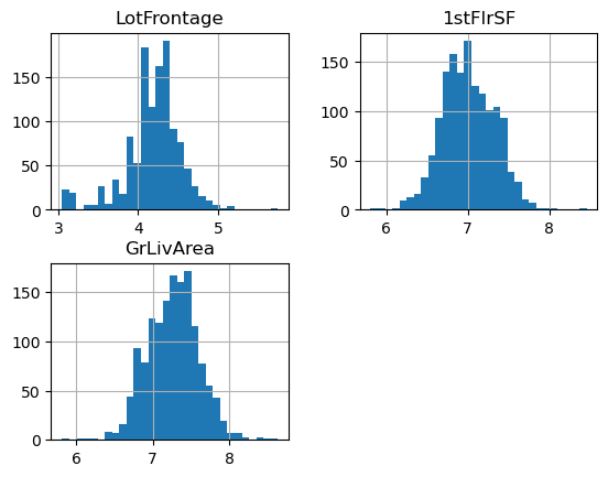
The distribution of the variables are now more “Gaussian” looking.

Evaluating their relationship with the target.

# Plotting the original or transformed variables
# vs sale price, and see if there is a relationship

for var in ["LotFrontage", "1stFlrSF", "GrLivArea"]:

    plt.figure(figsize=(12, 4))

    # plot the original variable vs sale price
    plt.subplot(1, 2, 1)
    plt.scatter(data[var], np.log(data["SalePrice"]))
    plt.ylabel("Sale Price")
    plt.xlabel("Original " + var)

    # plot transformed variable vs sale price
    plt.subplot(1, 2, 2)
    plt.scatter(tmp[var], np.log(tmp["SalePrice"]))
    plt.ylabel("Sale Price")
    plt.xlabel("Transformed " + var)

    plt.show()

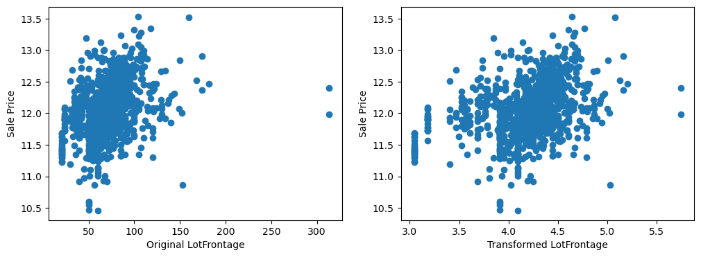
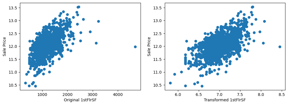
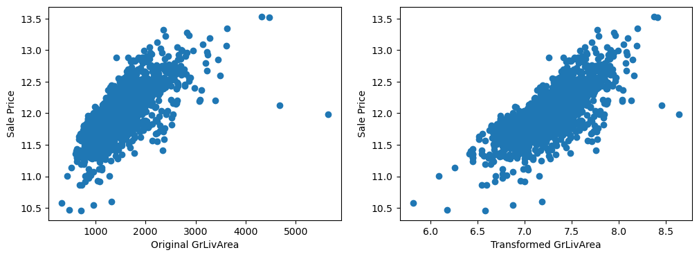
The transformed variables have a better spread of the values, which may in turn, help make better predictions.

Skewed variables

Transforming skewed vars into binary variables to check how predictive they are:

for var in skewed:

    tmp = data.copy()

    # map the variable values into 0 and 1
    tmp[var] = np.where(data[var] == 0, 0, 1)

    # determine mean sale price in the mapped values
    tmp = tmp.groupby(var)["SalePrice"].agg(["mean", "std"])

    # plot into a bar graph
    tmp.plot(
        kind="barh",
        y="mean",
        legend=False,
        xerr="std",
        title="Sale Price",
        color="green",
    )

    plt.show()

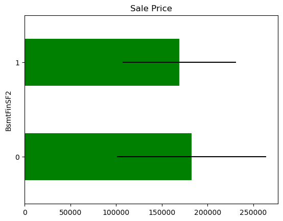
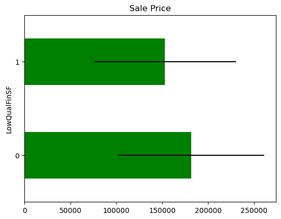
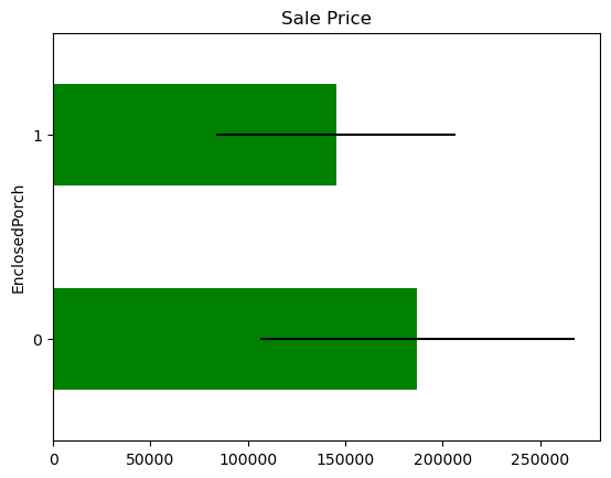
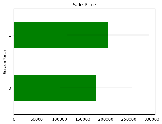
There seem to be a difference in Sale Price in the mapped values, but the confidence intervals overlap, so most likely this is not significant or predictive.

Categorical variables

Analysing the categorical variables present in the dataset.

print("Number of categorical variables: ", len(cat_vars))

Number of categorical variables:  44

# Visualising the values of the categorical variables
data[cat_vars].head()

	MSZoning	Street	Alley	LotShape	LandContour	Utilities	LotConfig	LandSlope	Neighborhood	Condition1	Condition2	BldgType	HouseStyle	RoofStyle	RoofMatl	Exterior1st	Exterior2nd	MasVnrType	ExterQual	ExterCond	Foundation	BsmtQual	BsmtCond	BsmtExposure	BsmtFinType1	BsmtFinType2	Heating	HeatingQC	CentralAir	Electrical	KitchenQual	Functional	FireplaceQu	GarageType	GarageFinish	GarageQual	GarageCond	PavedDrive	PoolQC	Fence	MiscFeature	SaleType	SaleCondition	MSSubClass
0	RL	Pave	NaN	Reg	Lvl	AllPub	Inside	Gtl	CollgCr	Norm	Norm	1Fam	2Story	Gable	CompShg	VinylSd	VinylSd	BrkFace	Gd	TA	PConc	Gd	TA	No	GLQ	Unf	GasA	Ex	Y	SBrkr	Gd	Typ	NaN	Attchd	RFn	TA	TA	Y	NaN	NaN	NaN	WD	Normal	60
1	RL	Pave	NaN	Reg	Lvl	AllPub	FR2	Gtl	Veenker	Feedr	Norm	1Fam	1Story	Gable	CompShg	MetalSd	MetalSd	None	TA	TA	CBlock	Gd	TA	Gd	ALQ	Unf	GasA	Ex	Y	SBrkr	TA	Typ	TA	Attchd	RFn	TA	TA	Y	NaN	NaN	NaN	WD	Normal	20
2	RL	Pave	NaN	IR1	Lvl	AllPub	Inside	Gtl	CollgCr	Norm	Norm	1Fam	2Story	Gable	CompShg	VinylSd	VinylSd	BrkFace	Gd	TA	PConc	Gd	TA	Mn	GLQ	Unf	GasA	Ex	Y	SBrkr	Gd	Typ	TA	Attchd	RFn	TA	TA	Y	NaN	NaN	NaN	WD	Normal	60
3	RL	Pave	NaN	IR1	Lvl	AllPub	Corner	Gtl	Crawfor	Norm	Norm	1Fam	2Story	Gable	CompShg	Wd Sdng	Wd Shng	None	TA	TA	BrkTil	TA	Gd	No	ALQ	Unf	GasA	Gd	Y	SBrkr	Gd	Typ	Gd	Detchd	Unf	TA	TA	Y	NaN	NaN	NaN	WD	Abnorml	70
4	RL	Pave	NaN	IR1	Lvl	AllPub	FR2	Gtl	NoRidge	Norm	Norm	1Fam	2Story	Gable	CompShg	VinylSd	VinylSd	BrkFace	Gd	TA	PConc	Gd	TA	Av	GLQ	Unf	GasA	Ex	Y	SBrkr	Gd	Typ	TA	Attchd	RFn	TA	TA	Y	NaN	NaN	NaN	WD	Normal	60

Number of labels: cardinality

How many categories are present in each of the variables?

# counting unique categories with pandas unique()
# and then plotting them in descending order

data[cat_vars].nunique().sort_values(ascending=False).plot.bar(figsize=(12, 5))

<AxesSubplot: >

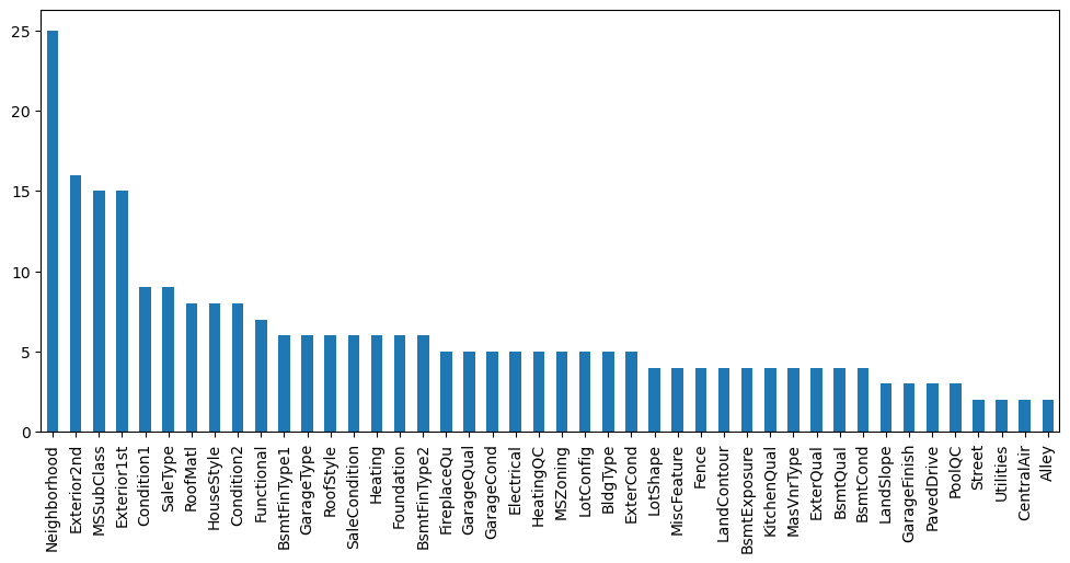
All the categorical variables show low cardinality, this means that they have only few different labels.

Quality variables

There are a number of variables that refer to the quality of some aspect of the house, for example the garage, or the fence, or the kitchen. Replace these categories by numbers increasing with the quality of the place or room.

The mappings can be obtained from the Kaggle Website. One example:

• Ex = Excellent

• Gd = Good

• TA = Average/Typical

• Fa = Fair

• Po = Poor

# Re-mapping strings to number, which determine quality

qual_mappings = {
    "Po": 1,
    "Fa": 2,
    "TA": 3,
    "Gd": 4,
    "Ex": 5,
    "Missing": 0,
    "NA": 0,
}

qual_vars = [
    "ExterQual",
    "ExterCond",
    "BsmtQual",
    "BsmtCond",
    "HeatingQC",
    "KitchenQual",
    "FireplaceQu",
    "GarageQual",
    "GarageCond",
]

for var in qual_vars:
    data[var] = data[var].map(qual_mappings)

exposure_mappings = {"No": 1, "Mn": 2, "Av": 3, "Gd": 4, "Missing": 0, "NA": 0}

var = "BsmtExposure"

data[var] = data[var].map(exposure_mappings)

finish_mappings = {
    "Missing": 0,
    "NA": 0,
    "Unf": 1,
    "LwQ": 2,
    "Rec": 3,
    "BLQ": 4,
    "ALQ": 5,
    "GLQ": 6,
}

finish_vars = ["BsmtFinType1", "BsmtFinType2"]

for var in finish_vars:
    data[var] = data[var].map(finish_mappings)

garage_mappings = {"Missing": 0, "NA": 0, "Unf": 1, "RFn": 2, "Fin": 3}

var = "GarageFinish"

data[var] = data[var].map(garage_mappings)

fence_mappings = {
    "Missing": 0,
    "NA": 0,
    "MnWw": 1,
    "GdWo": 2,
    "MnPrv": 3,
    "GdPrv": 4,
}

var = "Fence"

data[var] = data[var].map(fence_mappings)

# capture all quality variables

qual_vars = qual_vars + finish_vars + ["BsmtExposure", "GarageFinish", "Fence"]

# Plotting the house mean sale price based on the quality of the
# various attributes

for var in qual_vars:
    # boxplot with Catplot
    sns.catplot(
        x=var, y="SalePrice", data=data, kind="box", height=4, aspect=1.5
    )
    # data points to boxplot with stripplot
    sns.stripplot(
        x=var, y="SalePrice", data=data, jitter=0.1, alpha=0.3, color="k"
    )
    plt.show()

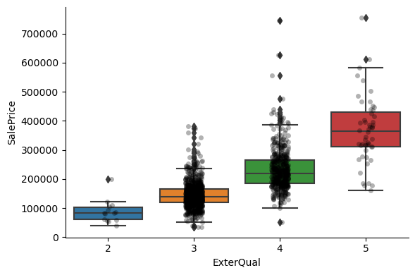
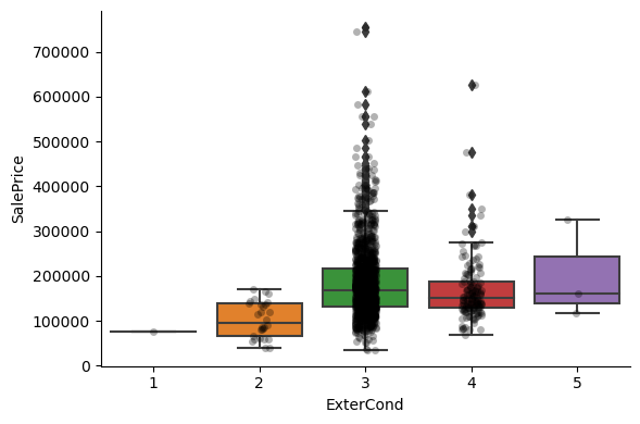
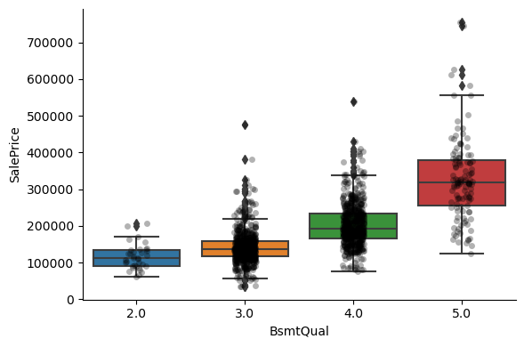
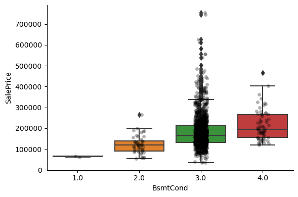
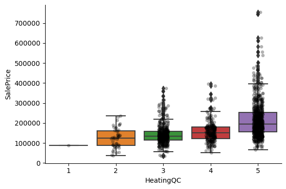
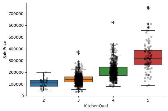
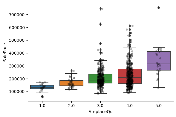
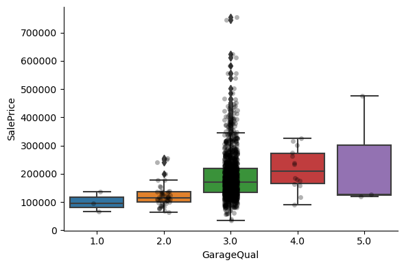
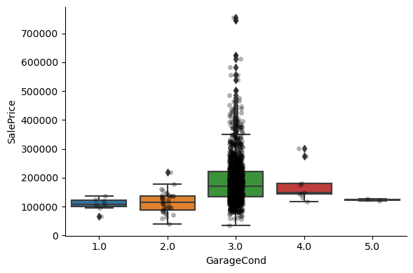
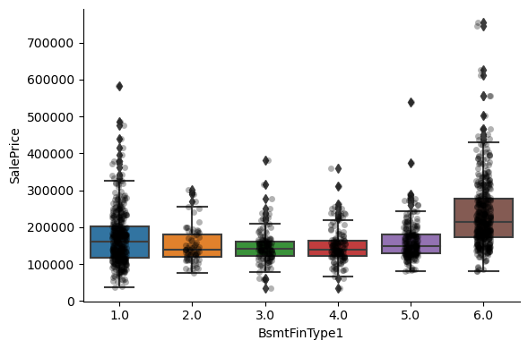
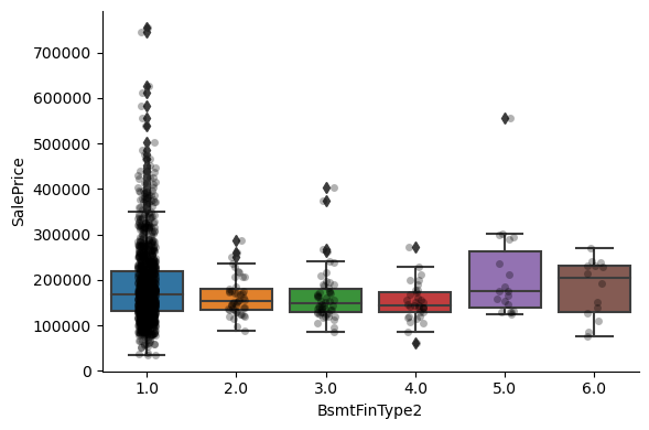
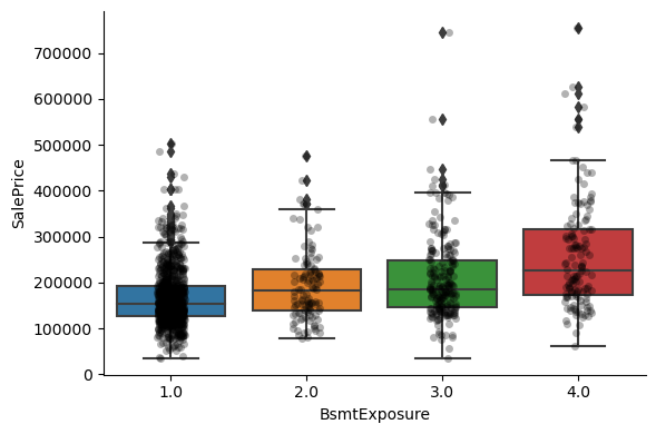
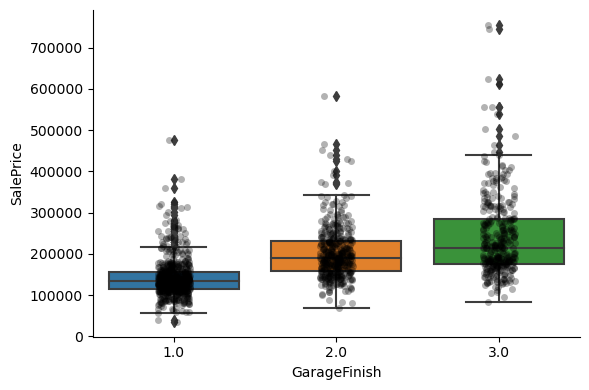
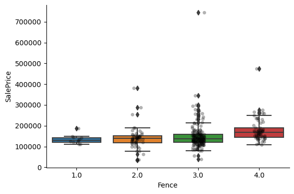
For most attributes, the increase in the house price with the value of the variable, is quite clear.

# Capturing the remaining categorical variables
# (those that we did not re-map)
cat_others = [var for var in cat_vars if var not in qual_vars]

len(cat_others)

30

Rare labels

Investigating if there are labels that are present only in a small number of houses:

def analyse_rare_labels(df, var, rare_perc):
    df = df.copy()

    # determine the % of observations per category
    temp = df.groupby(var)["SalePrice"].count() / len(df)

    # return categories that are rare
    return temp[temp < rare_perc]


# print categories that are present in less than
# 1 % of the observations

for var in cat_others:
    print(analyse_rare_labels(data, var, 0.01))
    print()

MSZoning
C (all)    0.006849
Name: SalePrice, dtype: float64

Street
Grvl    0.00411
Name: SalePrice, dtype: float64

Series([], Name: SalePrice, dtype: float64)

LotShape
IR3    0.006849
Name: SalePrice, dtype: float64

Series([], Name: SalePrice, dtype: float64)

Utilities
NoSeWa    0.000685
Name: SalePrice, dtype: float64

LotConfig
FR3    0.00274
Name: SalePrice, dtype: float64

LandSlope
Sev    0.008904
Name: SalePrice, dtype: float64

Neighborhood
Blueste    0.001370
NPkVill    0.006164
Veenker    0.007534
Name: SalePrice, dtype: float64

Condition1
PosA    0.005479
RRAe    0.007534
RRNe    0.001370
RRNn    0.003425
Name: SalePrice, dtype: float64

Condition2
Artery    0.001370
Feedr     0.004110
PosA      0.000685
PosN      0.001370
RRAe      0.000685
RRAn      0.000685
RRNn      0.001370
Name: SalePrice, dtype: float64

Series([], Name: SalePrice, dtype: float64)

HouseStyle
1.5Unf    0.009589
2.5Fin    0.005479
2.5Unf    0.007534
Name: SalePrice, dtype: float64

RoofStyle
Flat       0.008904
Gambrel    0.007534
Mansard    0.004795
Shed       0.001370
Name: SalePrice, dtype: float64

RoofMatl
ClyTile    0.000685
Membran    0.000685
Metal      0.000685
Roll       0.000685
Tar&Grv    0.007534
WdShake    0.003425
WdShngl    0.004110
Name: SalePrice, dtype: float64

Exterior1st
AsphShn    0.000685
BrkComm    0.001370
CBlock     0.000685
ImStucc    0.000685
Stone      0.001370
Name: SalePrice, dtype: float64

Exterior2nd
AsphShn    0.002055
Brk Cmn    0.004795
CBlock     0.000685
ImStucc    0.006849
Other      0.000685
Stone      0.003425
Name: SalePrice, dtype: float64

Series([], Name: SalePrice, dtype: float64)

Foundation
Stone    0.004110
Wood     0.002055
Name: SalePrice, dtype: float64

Heating
Floor    0.000685
Grav     0.004795
OthW     0.001370
Wall     0.002740
Name: SalePrice, dtype: float64

Series([], Name: SalePrice, dtype: float64)

Electrical
FuseP    0.002055
Mix      0.000685
Name: SalePrice, dtype: float64

Functional
Maj1    0.009589
Maj2    0.003425
Sev     0.000685
Name: SalePrice, dtype: float64

GarageType
2Types     0.004110
CarPort    0.006164
Name: SalePrice, dtype: float64

Series([], Name: SalePrice, dtype: float64)

PoolQC
Ex    0.001370
Fa    0.001370
Gd    0.002055
Name: SalePrice, dtype: float64

MiscFeature
Gar2    0.001370
Othr    0.001370
TenC    0.000685
Name: SalePrice, dtype: float64

SaleType
CWD      0.002740
Con      0.001370
ConLD    0.006164
ConLI    0.003425
ConLw    0.003425
Oth      0.002055
Name: SalePrice, dtype: float64

SaleCondition
AdjLand    0.002740
Alloca     0.008219
Name: SalePrice, dtype: float64

MSSubClass
40     0.002740
45     0.008219
180    0.006849
Name: SalePrice, dtype: float64

Some categorical variables show multiple labels that are present in less than 1% of the houses.

Labels that are under-represented in the dataset tend to cause over-fitting of machine learning models.

Removing.

Exploring the relationship between the categories of the different variables and the house sale price:

for var in cat_others:
    # make boxplot with Catplot
    sns.catplot(
        x=var, y="SalePrice", data=data, kind="box", height=4, aspect=1.5
    )
    # add data points to boxplot with stripplot
    sns.stripplot(
        x=var, y="SalePrice", data=data, jitter=0.1, alpha=0.3, color="k"
    )
    plt.show()

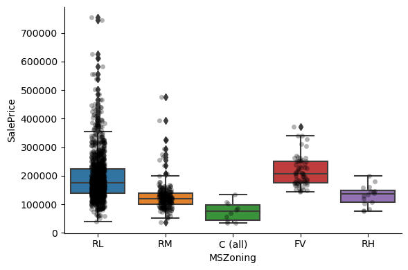
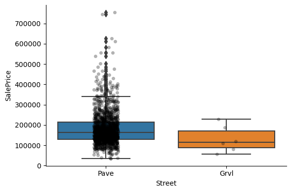
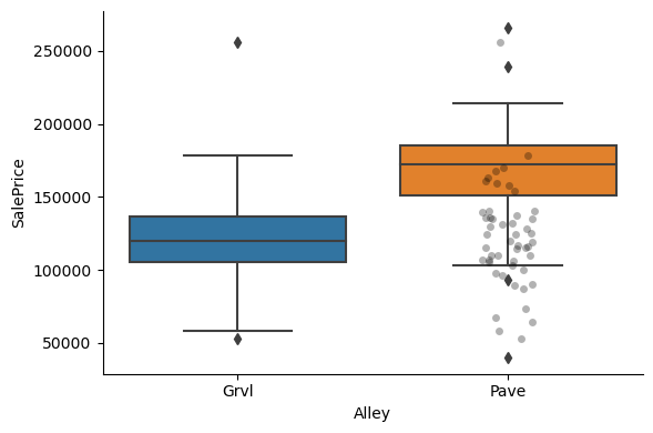
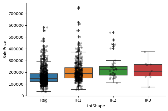
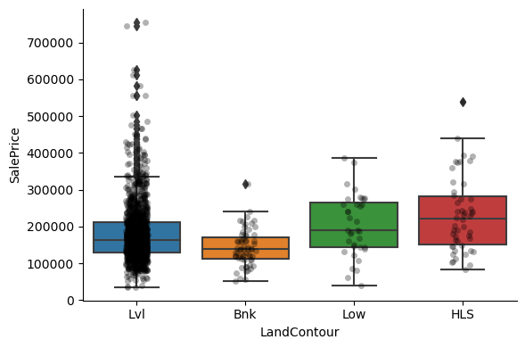
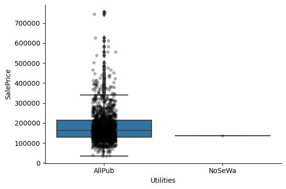
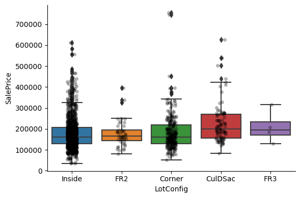
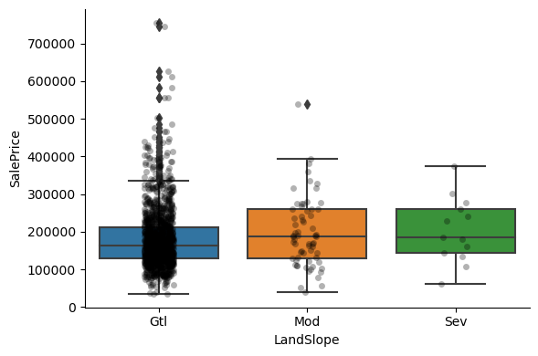
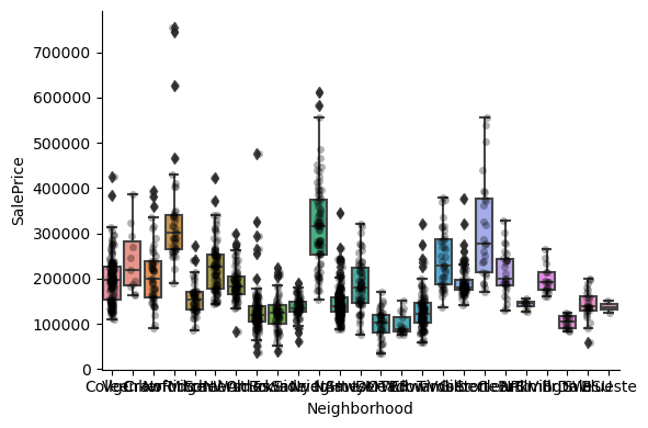
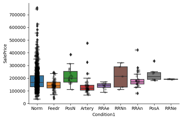
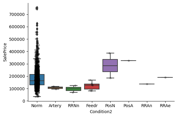
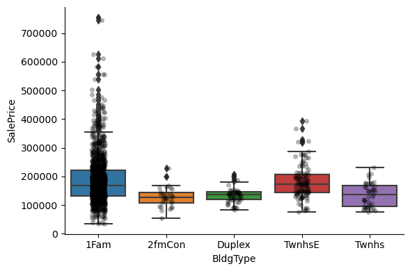
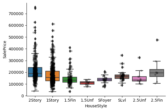
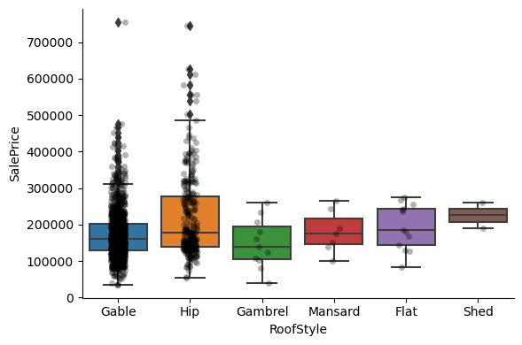
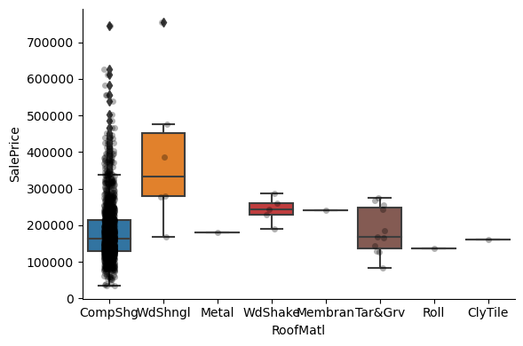
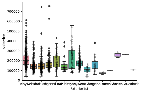
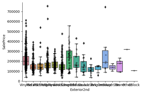
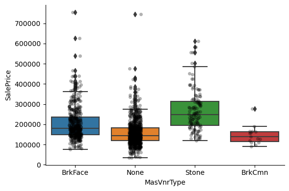
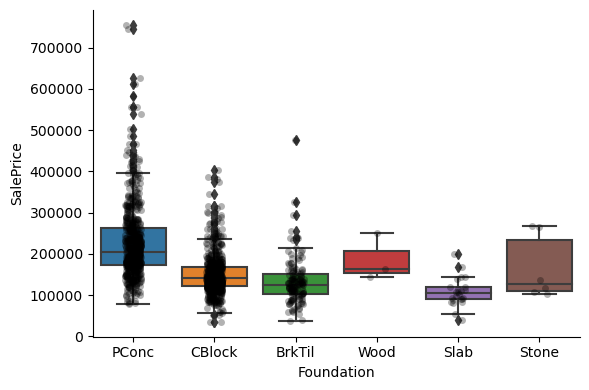
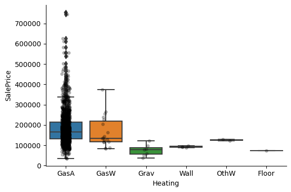
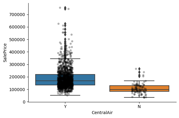
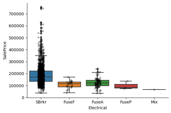
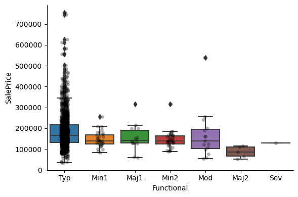
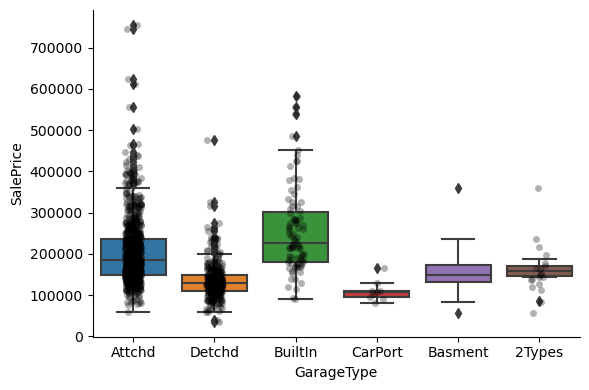
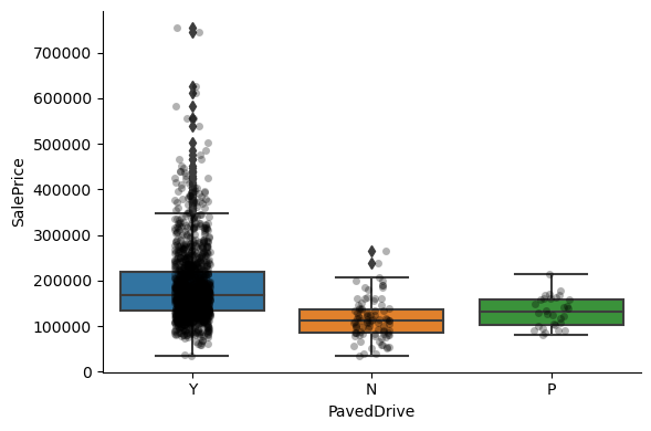
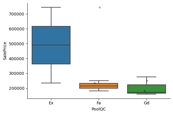
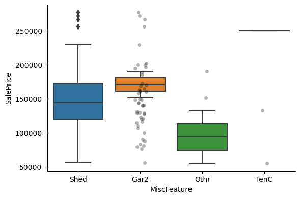
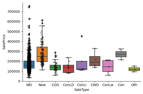
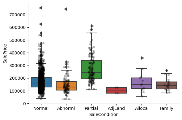
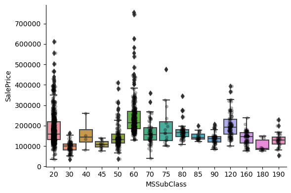
Clearly, the categories give information on the SalePrice, as different categories show different median sale prices.

Disclaimer:

There is certainly more that can be done to understand the nature of this data and the relationship of these variables with the target, SalePrice. And also about the distribution of the variables themselves.

Additional Resources

• Feature Engineering for Machine Learning - Online Course

• Packt Feature Engineering Cookbook - Book

• Predict house price with Feature-engine - Kaggle kernel

• Comprehensive data exploration with Python - Kaggle kernel

• How I made top 0.3% on a Kaggle competition - Kaggle kernel