Ames Housing Model Training

Using the transformed datasets and the selected variables saved in the previous notebooks to try a model.

Reproducibility: Setting the seed

With the aim to ensure reproducibility between runs of the same notebook, and between the research and production environment, for each step that includes some element of randomness, it is extremely important that the seed is set.

Libraries and packages

# to handle datasets
import pandas as pd
import numpy as np

# for plotting
import matplotlib.pyplot as plt

# to save the model
import joblib

# to build the model
from sklearn.linear_model import Lasso

# to evaluate the model
from sklearn.metrics import mean_squared_error, r2_score

# to visualise al the columns in the dataframe
pd.pandas.set_option("display.max_columns", None)

Paths

# Path to datasets directory
data_path = "./datasets"
# Path to assets directory (for saving results to)
assets_path = "./assets"

Loading dataset

# Load the train and test set with the engineered variables
X_train = pd.read_csv(f"{data_path}/xtrain.csv")
X_test = pd.read_csv(f"{data_path}/xtest.csv")

X_train.head()

	MSSubClass	MSZoning	LotFrontage	LotArea	Street	Alley	LotShape	LandContour	Utilities	LotConfig	LandSlope	Neighborhood	Condition1	Condition2	BldgType	HouseStyle	OverallQual	OverallCond	YearBuilt	YearRemodAdd	RoofStyle	RoofMatl	Exterior1st	Exterior2nd	MasVnrType	MasVnrArea	ExterQual	ExterCond	Foundation	BsmtQual	BsmtCond	BsmtExposure	BsmtFinType1	BsmtFinSF1	BsmtFinType2	BsmtFinSF2	BsmtUnfSF	TotalBsmtSF	Heating	HeatingQC	CentralAir	Electrical	1stFlrSF	2ndFlrSF	LowQualFinSF	GrLivArea	BsmtFullBath	BsmtHalfBath	FullBath	HalfBath	BedroomAbvGr	KitchenAbvGr	KitchenQual	TotRmsAbvGrd	Functional	Fireplaces	FireplaceQu	GarageType	GarageYrBlt	GarageFinish	GarageCars	GarageArea	GarageQual	GarageCond	PavedDrive	WoodDeckSF	OpenPorchSF	EnclosedPorch	3SsnPorch	ScreenPorch	PoolArea	PoolQC	Fence	MiscFeature	MiscVal	MoSold	SaleType	SaleCondition	LotFrontage_na	MasVnrArea_na	GarageYrBlt_na
0	0.750000	0.75	0.461171	0.366365	1.0	1.0	0.333333	1.000000	1.0	0.0	0.0	0.863636	0.4	1.0	0.75	0.6	0.777778	0.50	0.014706	0.049180	0.0	0.0	1.0	1.0	0.333333	0.00000	0.666667	0.5	1.0	0.666667	0.666667	0.666667	1.0	0.002835	0.0	0.0	0.673479	0.239935	1.0	1.00	1.0	1.0	0.559760	0.0	0.0	0.523250	0.000000	0.0	0.666667	0.0	0.375	0.333333	0.666667	0.416667	1.0	0.000000	0.0	0.75	0.018692	1.0	0.75	0.430183	0.5	0.5	1.0	0.116686	0.032907	0.0	0.0	0.0	0.0	0.0	0.00	1.0	0.0	0.545455	0.666667	0.75	0.0	0.0	0.0
1	0.750000	0.75	0.456066	0.388528	1.0	1.0	0.333333	0.333333	1.0	0.0	0.0	0.363636	0.4	1.0	0.75	0.6	0.444444	0.75	0.360294	0.049180	0.0	0.0	0.6	0.6	0.666667	0.03375	0.666667	0.5	0.5	0.333333	0.666667	0.000000	0.8	0.142807	0.0	0.0	0.114724	0.172340	1.0	1.00	1.0	1.0	0.434539	0.0	0.0	0.406196	0.333333	0.0	0.333333	0.5	0.375	0.333333	0.666667	0.250000	1.0	0.000000	0.0	0.75	0.457944	0.5	0.25	0.220028	0.5	0.5	1.0	0.000000	0.000000	0.0	0.0	0.0	0.0	0.0	0.75	1.0	0.0	0.636364	0.666667	0.75	0.0	0.0	0.0
2	0.916667	0.75	0.394699	0.336782	1.0	1.0	0.000000	0.333333	1.0	0.0	0.0	0.954545	0.4	1.0	1.00	0.6	0.888889	0.50	0.036765	0.098361	1.0	0.0	0.3	0.2	0.666667	0.25750	1.000000	0.5	1.0	1.000000	0.666667	0.000000	1.0	0.080794	0.0	0.0	0.601951	0.286743	1.0	1.00	1.0	1.0	0.627205	0.0	0.0	0.586296	0.333333	0.0	0.666667	0.0	0.250	0.333333	1.000000	0.333333	1.0	0.333333	0.8	0.75	0.046729	0.5	0.50	0.406206	0.5	0.5	1.0	0.228705	0.149909	0.0	0.0	0.0	0.0	0.0	0.00	1.0	0.0	0.090909	0.666667	0.75	0.0	0.0	0.0
3	0.750000	0.75	0.445002	0.482280	1.0	1.0	0.666667	0.666667	1.0	0.0	0.0	0.454545	0.4	1.0	0.75	0.6	0.666667	0.50	0.066176	0.163934	0.0	0.0	1.0	1.0	0.333333	0.00000	0.666667	0.5	1.0	0.666667	0.666667	1.000000	1.0	0.255670	0.0	0.0	0.018114	0.242553	1.0	1.00	1.0	1.0	0.566920	0.0	0.0	0.529943	0.333333	0.0	0.666667	0.0	0.375	0.333333	0.666667	0.250000	1.0	0.333333	0.4	0.75	0.084112	0.5	0.50	0.362482	0.5	0.5	1.0	0.469078	0.045704	0.0	0.0	0.0	0.0	0.0	0.00	1.0	0.0	0.636364	0.666667	0.75	1.0	0.0	0.0
4	0.750000	0.75	0.577658	0.391756	1.0	1.0	0.333333	0.333333	1.0	0.0	0.0	0.363636	0.4	1.0	0.75	0.6	0.555556	0.50	0.323529	0.737705	0.0	0.0	0.6	0.7	0.666667	0.17000	0.333333	0.5	0.5	0.333333	0.666667	0.000000	0.6	0.086818	0.0	0.0	0.434278	0.233224	1.0	0.75	1.0	1.0	0.549026	0.0	0.0	0.513216	0.000000	0.0	0.666667	0.0	0.375	0.333333	0.333333	0.416667	1.0	0.333333	0.8	0.75	0.411215	0.5	0.50	0.406206	0.5	0.5	1.0	0.000000	0.000000	0.0	1.0	0.0	0.0	0.0	0.00	1.0	0.0	0.545455	0.666667	0.75	0.0	0.0	0.0

# load the target (remember that the target is log transformed)
y_train = pd.read_csv(f"{data_path}/ytrain.csv")
y_test = pd.read_csv(f"{data_path}/ytest.csv")

y_train.head()

	SalePrice
0	12.211060
1	11.887931
2	12.675764
3	12.278393
4	12.103486

# load the pre-selected features
# ==============================

features = pd.read_csv(f"{data_path}/selected_features.csv")
features = features["0"].to_list()

# display final feature set
features

['MSSubClass',
 'MSZoning',
 'LotArea',
 'LotShape',
 'LandContour',
 'LotConfig',
 'Neighborhood',
 'OverallQual',
 'OverallCond',
 'YearRemodAdd',
 'RoofStyle',
 'Exterior1st',
 'ExterQual',
 'Foundation',
 'BsmtQual',
 'BsmtExposure',
 'BsmtFinType1',
 'HeatingQC',
 'CentralAir',
 '1stFlrSF',
 '2ndFlrSF',
 'GrLivArea',
 'BsmtFullBath',
 'FullBath',
 'HalfBath',
 'KitchenQual',
 'TotRmsAbvGrd',
 'Functional',
 'Fireplaces',
 'FireplaceQu',
 'GarageFinish',
 'GarageCars',
 'PavedDrive',
 'WoodDeckSF',
 'ScreenPorch',
 'SaleCondition']

# reduce the train and test set to the selected features
X_train = X_train[features]
X_test = X_test[features]

Regularised linear regression: Lasso

*** set the seed ***

# set up the model
lin_model = Lasso(alpha=0.001, random_state=0)

# train the model
lin_model.fit(X_train, y_train)

Lasso(alpha=0.001, random_state=0)

In a Jupyter environment, please rerun this cell to show the HTML representation or trust the notebook.
On GitHub, the HTML representation is unable to render, please try loading this page with nbviewer.org.

# evaluate the model:
# ====================

# The output was log transformed in the feature engineering
# notebook.

# In order to get the true performance of the Lasso, transform
# the target and the predictions back to the original house
# prices values.

# Evaluate performance using the mean squared error and
# the root of the mean squared error and r2

# Making predictions for train set
pred = lin_model.predict(X_train)

# mse, rmse and r2
print(
    "train mse: {}".format(
        int(mean_squared_error(np.exp(y_train), np.exp(pred)))
    )
)
print(
    "train rmse: {}".format(
        int(mean_squared_error(np.exp(y_train), np.exp(pred), squared=False))
    )
)
print("train r2: {}".format(r2_score(np.exp(y_train), np.exp(pred))))
print()

# Making predictions for test set
pred = lin_model.predict(X_test)

# mse, rmse and r2
print(
    "test mse: {}".format(
        int(mean_squared_error(np.exp(y_test), np.exp(pred)))
    )
)
print(
    "test rmse: {}".format(
        int(mean_squared_error(np.exp(y_test), np.exp(pred), squared=False))
    )
)
print("test r2: {}".format(r2_score(np.exp(y_test), np.exp(pred))))
print()

print("Average house price: ", int(np.exp(y_train).median()))

train mse: 772198334
train rmse: 27788
train r2: 0.8763262128412839

test mse: 1077066272
test rmse: 32818
test r2: 0.8432700518729047

Average house price:  162999

# Evaluate predictions wrt to the real sale price
plt.scatter(y_test, lin_model.predict(X_test))
plt.xlabel("True House Price")
plt.ylabel("Predicted House Price")
plt.title("Evaluation of Lasso Predictions")

Text(0.5, 1.0, 'Evaluation of Lasso Predictions')

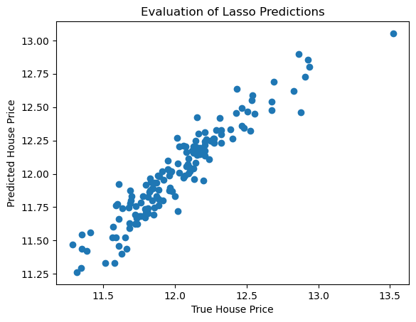
The model is doing a good job at estimating house prices.

y_test.reset_index(drop=True)

	SalePrice
0	12.209188
1	11.798104
2	11.608236
3	12.165251
4	11.385092
...	...
141	11.884489
142	12.287653
143	11.921718
144	11.598727
145	12.017331

146 rows × 1 columns

# Evaluating the distribution of the errors:
# they should be fairly normally distributed
y_test.reset_index(drop=True, inplace=True)

preds = pd.Series(lin_model.predict(X_test))
preds

0      12.175793
1      11.917238
2      11.662980
3      12.303104
4      11.423063
         ...    
141    11.763792
142    12.329463
143    11.954652
144    11.772995
145    12.077226
Length: 146, dtype: float64

# Evaluating the distribution of the errors:
# they should be fairly normally distributed

errors = y_test["SalePrice"] - preds
errors.hist(bins=30)
plt.show()

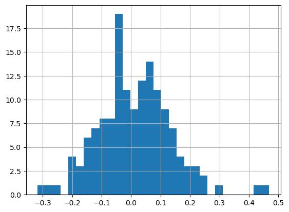
The distribution of the errors follows quite closely a gaussian distribution. That suggests that the model is doing a good job as well.

Feature importance

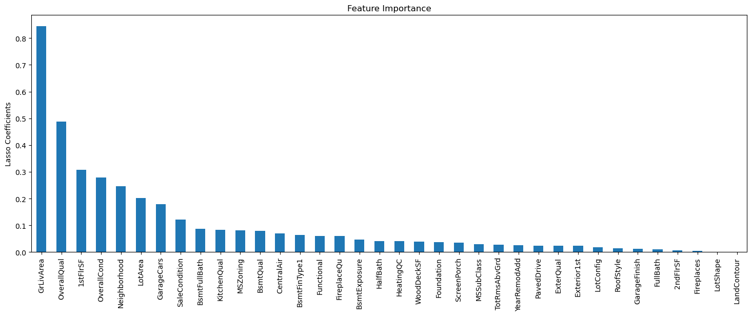
# Just for fun, feature importance
importance = pd.Series(np.abs(lin_model.coef_.ravel()))
importance.index = features
importance.sort_values(inplace=True, ascending=False)
importance.plot.bar(figsize=(18, 6))
plt.ylabel("Lasso Coefficients")
plt.title("Feature Importance")

Text(0.5, 1.0, 'Feature Importance')

Save the Model

# Save the model to be able to score new data

joblib.dump(lin_model, f"{data_path}/linear_regression.joblib")

['./datasets/linear_regression.joblib']