Feature Engineering with Open-Source

In this notebook, the Feature Engineering Pipeline from the Housing Feature Engineering notebook of Machine Learning Preprocessing is used. The manually created functions are replaced by open-source classes.

1. Missing values

2. Temporal variables

3. Non-Gaussian distributed variables

4. Categorical variables: remove rare labels

5. Categorical variables: convert strings to numbers

6. Standardize the values of the variables to the same range

With the aim to ensure reproducibility between runs of the same notebook, and between the research and production environment, for each step that includes some element of randomness, it is extremely important that the seed is set.

# data manipulation and plotting
import pandas as pd
import numpy as np
import matplotlib.pyplot as plt

# from Scikit-learn
from sklearn.model_selection import train_test_split
from sklearn.preprocessing import MinMaxScaler, Binarizer

# from feature-engine
from feature_engine.imputation import (
    AddMissingIndicator,
    MeanMedianImputer,
    CategoricalImputer,
)

from feature_engine.encoding import (
    RareLabelEncoder,
    OrdinalEncoder,
)

from feature_engine.transformation import (
    LogTransformer,
    YeoJohnsonTransformer,
)

from feature_engine.selection import DropFeatures
from feature_engine.wrappers import SklearnTransformerWrapper

# to visualise al the columns in the dataframe
pd.pandas.set_option("display.max_columns", None)

Paths

# Path to datasets directory
data_path = "./datasets"
# Path to assets directory (for saving results to)
assets_path = "./assets"

Loading dataset

# load dataset
data = pd.read_csv(f"{data_path}/train.csv")

# rows and columns of the data
print(data.shape)

# visualise the dataset
data.head()

(1460, 81)

	Id	MSSubClass	MSZoning	LotFrontage	LotArea	Street	Alley	LotShape	LandContour	Utilities	LotConfig	LandSlope	Neighborhood	Condition1	Condition2	BldgType	HouseStyle	OverallQual	OverallCond	YearBuilt	YearRemodAdd	RoofStyle	RoofMatl	Exterior1st	Exterior2nd	MasVnrType	MasVnrArea	ExterQual	ExterCond	Foundation	BsmtQual	BsmtCond	BsmtExposure	BsmtFinType1	BsmtFinSF1	BsmtFinType2	BsmtFinSF2	BsmtUnfSF	TotalBsmtSF	Heating	HeatingQC	CentralAir	Electrical	1stFlrSF	2ndFlrSF	LowQualFinSF	GrLivArea	BsmtFullBath	BsmtHalfBath	FullBath	HalfBath	BedroomAbvGr	KitchenAbvGr	KitchenQual	TotRmsAbvGrd	Functional	Fireplaces	FireplaceQu	GarageType	GarageYrBlt	GarageFinish	GarageCars	GarageArea	GarageQual	GarageCond	PavedDrive	WoodDeckSF	OpenPorchSF	EnclosedPorch	3SsnPorch	ScreenPorch	PoolArea	PoolQC	Fence	MiscFeature	MiscVal	MoSold	YrSold	SaleType	SaleCondition	SalePrice
0	1	60	RL	65.0	8450	Pave	NaN	Reg	Lvl	AllPub	Inside	Gtl	CollgCr	Norm	Norm	1Fam	2Story	7	5	2003	2003	Gable	CompShg	VinylSd	VinylSd	BrkFace	196.0	Gd	TA	PConc	Gd	TA	No	GLQ	706	Unf	0	150	856	GasA	Ex	Y	SBrkr	856	854	0	1710	1	0	2	1	3	1	Gd	8	Typ	0	NaN	Attchd	2003.0	RFn	2	548	TA	TA	Y	0	61	0	0	0	0	NaN	NaN	NaN	0	2	2008	WD	Normal	208500
1	2	20	RL	80.0	9600	Pave	NaN	Reg	Lvl	AllPub	FR2	Gtl	Veenker	Feedr	Norm	1Fam	1Story	6	8	1976	1976	Gable	CompShg	MetalSd	MetalSd	None	0.0	TA	TA	CBlock	Gd	TA	Gd	ALQ	978	Unf	0	284	1262	GasA	Ex	Y	SBrkr	1262	0	0	1262	0	1	2	0	3	1	TA	6	Typ	1	TA	Attchd	1976.0	RFn	2	460	TA	TA	Y	298	0	0	0	0	0	NaN	NaN	NaN	0	5	2007	WD	Normal	181500
2	3	60	RL	68.0	11250	Pave	NaN	IR1	Lvl	AllPub	Inside	Gtl	CollgCr	Norm	Norm	1Fam	2Story	7	5	2001	2002	Gable	CompShg	VinylSd	VinylSd	BrkFace	162.0	Gd	TA	PConc	Gd	TA	Mn	GLQ	486	Unf	0	434	920	GasA	Ex	Y	SBrkr	920	866	0	1786	1	0	2	1	3	1	Gd	6	Typ	1	TA	Attchd	2001.0	RFn	2	608	TA	TA	Y	0	42	0	0	0	0	NaN	NaN	NaN	0	9	2008	WD	Normal	223500
3	4	70	RL	60.0	9550	Pave	NaN	IR1	Lvl	AllPub	Corner	Gtl	Crawfor	Norm	Norm	1Fam	2Story	7	5	1915	1970	Gable	CompShg	Wd Sdng	Wd Shng	None	0.0	TA	TA	BrkTil	TA	Gd	No	ALQ	216	Unf	0	540	756	GasA	Gd	Y	SBrkr	961	756	0	1717	1	0	1	0	3	1	Gd	7	Typ	1	Gd	Detchd	1998.0	Unf	3	642	TA	TA	Y	0	35	272	0	0	0	NaN	NaN	NaN	0	2	2006	WD	Abnorml	140000
4	5	60	RL	84.0	14260	Pave	NaN	IR1	Lvl	AllPub	FR2	Gtl	NoRidge	Norm	Norm	1Fam	2Story	8	5	2000	2000	Gable	CompShg	VinylSd	VinylSd	BrkFace	350.0	Gd	TA	PConc	Gd	TA	Av	GLQ	655	Unf	0	490	1145	GasA	Ex	Y	SBrkr	1145	1053	0	2198	1	0	2	1	4	1	Gd	9	Typ	1	TA	Attchd	2000.0	RFn	3	836	TA	TA	Y	192	84	0	0	0	0	NaN	NaN	NaN	0	12	2008	WD	Normal	250000

Separate dataset into train and test

Feature engineering techniques:

• mean

• mode

• exponents for the yeo-johnson

• category frequency

• and category to number mappings

Separating the data into train and test involves randomness, therefore, we need to set the seed.

# Separate into train and test set.
# Set the seed (random_state for this sklearn function)

X_train, X_test, y_train, y_test = train_test_split(
    data.drop(["Id", "SalePrice"], axis=1),  # predictive variables
    data["SalePrice"],  # target
    test_size=0.1,  # portion of dataset to allocate to test set
    random_state=0,  # we are setting the seed here
)

X_train.shape, X_test.shape

((1314, 79), (146, 79))

Target

Applying the logarithm

y_train = np.log(y_train)
y_test = np.log(y_test)

Missing values

Categorical variables

Replacing missing values with the string “missing” in variables with a lot of missing data.

Alternatively, replacing missing data with the most frequent category in those variables that contain fewer observations without values.

# identify the categorical variables (type object)

cat_vars = [var for var in data.columns if data[var].dtype == "O"]

# MSSubClass is also categorical by definition, despite its numeric values
# (you can find the definitions of the variables in the data_description.txt
# file available on Kaggle, in the same website where you downloaded the data)

# add MSSubClass to the list of categorical variables
cat_vars = cat_vars + ["MSSubClass"]

# cast all variables as categorical
X_train[cat_vars] = X_train[cat_vars].astype("O")
X_test[cat_vars] = X_test[cat_vars].astype("O")

# number of categorical variables
len(cat_vars)

44

# make a list of the categorical variables that contain missing values
cat_vars_with_na = [var for var in cat_vars if X_train[var].isnull().sum() > 0]

# print percentage of missing values per variable
X_train[cat_vars_with_na].isnull().mean().sort_values(ascending=False)

PoolQC          0.995434
MiscFeature     0.961187
Alley           0.938356
Fence           0.814307
FireplaceQu     0.472603
GarageType      0.056317
GarageFinish    0.056317
GarageQual      0.056317
GarageCond      0.056317
BsmtExposure    0.025114
BsmtFinType2    0.025114
BsmtQual        0.024353
BsmtCond        0.024353
BsmtFinType1    0.024353
MasVnrType      0.004566
Electrical      0.000761
dtype: float64

# variables to impute with the string missing
with_string_missing = [
    var for var in cat_vars_with_na if X_train[var].isnull().mean() > 0.1
]

# variables to impute with the most frequent category
with_frequent_category = [
    var for var in cat_vars_with_na if X_train[var].isnull().mean() < 0.1
]

# print the values here, because it makes it easier for later
# when we need to add this values to a config file for deployment

with_string_missing

['Alley', 'FireplaceQu', 'PoolQC', 'Fence', 'MiscFeature']

with_frequent_category

['MasVnrType',
 'BsmtQual',
 'BsmtCond',
 'BsmtExposure',
 'BsmtFinType1',
 'BsmtFinType2',
 'Electrical',
 'GarageType',
 'GarageFinish',
 'GarageQual',
 'GarageCond']

# replace missing values with new label: "Missing"

# set up the class
cat_imputer_missing = CategoricalImputer(
    imputation_method="missing", variables=with_string_missing
)

# fit the class to the train set
cat_imputer_missing.fit(X_train)

# the class learns and stores the parameters
cat_imputer_missing.imputer_dict_

{'Alley': 'Missing',
 'FireplaceQu': 'Missing',
 'PoolQC': 'Missing',
 'Fence': 'Missing',
 'MiscFeature': 'Missing'}

# replace NA by missing

# IMPORTANT: note that we could store this class with joblib
X_train = cat_imputer_missing.transform(X_train)
X_test = cat_imputer_missing.transform(X_test)

# replace missing values with most frequent category

# set up the class
cat_imputer_frequent = CategoricalImputer(
    imputation_method="frequent", variables=with_frequent_category
)

# fit the class to the train set
cat_imputer_frequent.fit(X_train)

# the class learns and stores the parameters
cat_imputer_frequent.imputer_dict_

{'MasVnrType': 'None',
 'BsmtQual': 'TA',
 'BsmtCond': 'TA',
 'BsmtExposure': 'No',
 'BsmtFinType1': 'Unf',
 'BsmtFinType2': 'Unf',
 'Electrical': 'SBrkr',
 'GarageType': 'Attchd',
 'GarageFinish': 'Unf',
 'GarageQual': 'TA',
 'GarageCond': 'TA'}

# replace NA by missing

# IMPORTANT: note that we could store this class with joblib
X_train = cat_imputer_frequent.transform(X_train)
X_test = cat_imputer_frequent.transform(X_test)

# check that we have no missing information in the engineered variables

X_train[cat_vars_with_na].isnull().sum()

Alley           0
MasVnrType      0
BsmtQual        0
BsmtCond        0
BsmtExposure    0
BsmtFinType1    0
BsmtFinType2    0
Electrical      0
FireplaceQu     0
GarageType      0
GarageFinish    0
GarageQual      0
GarageCond      0
PoolQC          0
Fence           0
MiscFeature     0
dtype: int64

# check that test set does not contain null values in the engineered variables
[var for var in cat_vars_with_na if X_test[var].isnull().sum() > 0]

[]

Numerical variables

To engineer missing values in numerical variables:

• add a binary missing indicator variable

• and then replace the missing values in the original variable with the mean

# identify the numerical variables

num_vars = [
    var
    for var in X_train.columns
    if var not in cat_vars and var != "SalePrice"
]

# number of numerical variables
len(num_vars)

35

# list with the numerical variables that contain missing values
vars_with_na = [var for var in num_vars if X_train[var].isnull().sum() > 0]

# print percentage of missing values per variable
X_train[vars_with_na].isnull().mean()

LotFrontage    0.177321
MasVnrArea     0.004566
GarageYrBlt    0.056317
dtype: float64

# print, makes life easier when wanting to create a config
vars_with_na

['LotFrontage', 'MasVnrArea', 'GarageYrBlt']

# add missing indicator
missing_ind = AddMissingIndicator(variables=vars_with_na)

missing_ind.fit(X_train)

X_train = missing_ind.transform(X_train)
X_test = missing_ind.transform(X_test)

# check the binary missing indicator variables
X_train[["LotFrontage_na", "MasVnrArea_na", "GarageYrBlt_na"]].head()

	LotFrontage_na	MasVnrArea_na	GarageYrBlt_na
930	0	0	0
656	0	0	0
45	0	0	0
1348	1	0	0
55	0	0	0

# replace missing data with the mean

# set the imputer
mean_imputer = MeanMedianImputer(
    imputation_method="mean", variables=vars_with_na
)

# learn and store parameters from train set
mean_imputer.fit(X_train)

# the stored parameters
mean_imputer.imputer_dict_

{'LotFrontage': 69.87974098057354,
 'MasVnrArea': 103.7974006116208,
 'GarageYrBlt': 1978.2959677419356}

X_train = mean_imputer.transform(X_train)
X_test = mean_imputer.transform(X_test)

# IMPORTANT: note that we can save the imputers with joblib

# check that we have no more missing values in the engineered variables
X_train[vars_with_na].isnull().sum()

LotFrontage    0
MasVnrArea     0
GarageYrBlt    0
dtype: int64

# check that test set does not contain null values in the engineered variables
[var for var in vars_with_na if X_test[var].isnull().sum() > 0]

[]

Temporal variables

Capture elapsed time

There is in Feature-engine 2 classes that allow for performing the 2 transformations below:

• CombineWithFeatureReference to capture elapsed time

• DropFeatures to drop the unwanted features

Doing the first one manually. For the second operation, using the DropFeatures class.

def elapsed_years(df, var):
    # capture difference between the year variable
    # and the year in which the house was sold
    df[var] = df["YrSold"] - df[var]
    return df

for var in ["YearBuilt", "YearRemodAdd", "GarageYrBlt"]:
    X_train = elapsed_years(X_train, var)
    X_test = elapsed_years(X_test, var)

# now drop YrSold
drop_features = DropFeatures(features_to_drop=["YrSold"])

X_train = drop_features.fit_transform(X_train)
X_test = drop_features.transform(X_test)

Numerical variable transformation

Logarithmic transformation

The numerical variables are not normally distributed.

We will transform the positive numerical variables with the logarithm in order to get a more Gaussian-like distribution.

log_transformer = LogTransformer(
    variables=["LotFrontage", "1stFlrSF", "GrLivArea"]
)

X_train = log_transformer.fit_transform(X_train)
X_test = log_transformer.transform(X_test)

# check that test set does not contain null values in the engineered variables
[
    var
    for var in ["LotFrontage", "1stFlrSF", "GrLivArea"]
    if X_test[var].isnull().sum() > 0
]

[]

# same for train set
[
    var
    for var in ["LotFrontage", "1stFlrSF", "GrLivArea"]
    if X_train[var].isnull().sum() > 0
]

[]

Yeo-Johnson transformation

Applying the Yeo-Johnson transformation to LotArea.

yeo_transformer = YeoJohnsonTransformer(variables=["LotArea"])

X_train = yeo_transformer.fit_transform(X_train)
X_test = yeo_transformer.transform(X_test)

# the learned parameter
yeo_transformer.lambda_dict_

{'LotArea': 0.017755573660304995}

# check absence of na in the train set
[var for var in X_train.columns if X_train[var].isnull().sum() > 0]

[]

# check absence of na in the test set
[var for var in X_train.columns if X_test[var].isnull().sum() > 0]

[]

Binarize skewed variables

A few variables were very skewed, transforming into binary variables.

Possibly using the Binarizer from Scikit-learn, in combination with the SklearnWrapper from Feature-engine to be able to apply the transformation only to a subset of features.

Going to do it manually, to give us another opportunity to code the class as an exercise.

skewed = [
    "BsmtFinSF2",
    "LowQualFinSF",
    "EnclosedPorch",
    "3SsnPorch",
    "ScreenPorch",
    "MiscVal",
]

binarizer = SklearnTransformerWrapper(
    transformer=Binarizer(threshold=0), variables=skewed
)


X_train = binarizer.fit_transform(X_train)
X_test = binarizer.transform(X_test)

X_train[skewed].head()

	BsmtFinSF2	LowQualFinSF	EnclosedPorch	3SsnPorch	ScreenPorch	MiscVal
930	0	0	0	0	0	0
656	0	0	0	0	0	0
45	0	0	0	0	0	0
1348	0	0	0	0	0	0
55	0	0	0	1	0	0

Categorical variables

Apply mappings

# re-map strings to number, which determine quality

qual_mappings = {
    "Po": 1,
    "Fa": 2,
    "TA": 3,
    "Gd": 4,
    "Ex": 5,
    "Missing": 0,
    "NA": 0,
}

qual_vars = [
    "ExterQual",
    "ExterCond",
    "BsmtQual",
    "BsmtCond",
    "HeatingQC",
    "KitchenQual",
    "FireplaceQu",
    "GarageQual",
    "GarageCond",
]

for var in qual_vars:
    X_train[var] = X_train[var].map(qual_mappings)
    X_test[var] = X_test[var].map(qual_mappings)

exposure_mappings = {"No": 1, "Mn": 2, "Av": 3, "Gd": 4}

var = "BsmtExposure"

X_train[var] = X_train[var].map(exposure_mappings)
X_test[var] = X_test[var].map(exposure_mappings)

finish_mappings = {
    "Missing": 0,
    "NA": 0,
    "Unf": 1,
    "LwQ": 2,
    "Rec": 3,
    "BLQ": 4,
    "ALQ": 5,
    "GLQ": 6,
}

finish_vars = ["BsmtFinType1", "BsmtFinType2"]

for var in finish_vars:
    X_train[var] = X_train[var].map(finish_mappings)
    X_test[var] = X_test[var].map(finish_mappings)

garage_mappings = {"Missing": 0, "NA": 0, "Unf": 1, "RFn": 2, "Fin": 3}

var = "GarageFinish"

X_train[var] = X_train[var].map(garage_mappings)
X_test[var] = X_test[var].map(garage_mappings)

fence_mappings = {
    "Missing": 0,
    "NA": 0,
    "MnWw": 1,
    "GdWo": 2,
    "MnPrv": 3,
    "GdPrv": 4,
}

var = "Fence"

X_train[var] = X_train[var].map(fence_mappings)
X_test[var] = X_test[var].map(fence_mappings)

# check absence of na in the train set
[var for var in X_train.columns if X_train[var].isnull().sum() > 0]

[]

Removing Rare Labels

Grouping the remaining categorical variables present in less than 1% of the observations. That is, all values of categorical variables that are shared by less than 1% of houses, will be replaced by the string “Rare”.

# capture all quality variables

qual_vars = qual_vars + finish_vars + ["BsmtExposure", "GarageFinish", "Fence"]

# capture the remaining categorical variables
# (those that we did not re-map)

cat_others = [var for var in cat_vars if var not in qual_vars]

len(cat_others)

30

cat_others

['MSZoning',
 'Street',
 'Alley',
 'LotShape',
 'LandContour',
 'Utilities',
 'LotConfig',
 'LandSlope',
 'Neighborhood',
 'Condition1',
 'Condition2',
 'BldgType',
 'HouseStyle',
 'RoofStyle',
 'RoofMatl',
 'Exterior1st',
 'Exterior2nd',
 'MasVnrType',
 'Foundation',
 'Heating',
 'CentralAir',
 'Electrical',
 'Functional',
 'GarageType',
 'PavedDrive',
 'PoolQC',
 'MiscFeature',
 'SaleType',
 'SaleCondition',
 'MSSubClass']

rare_encoder = RareLabelEncoder(tol=0.01, n_categories=1, variables=cat_others)

# find common labels
rare_encoder.fit(X_train)

# the common labels are stored, we can save the class
# and then use it later :)
rare_encoder.encoder_dict_

{'MSZoning': Index(['RL', 'RM', 'FV', 'RH'], dtype='object'),
 'Street': Index(['Pave'], dtype='object'),
 'Alley': Index(['Missing', 'Grvl', 'Pave'], dtype='object'),
 'LotShape': Index(['Reg', 'IR1', 'IR2'], dtype='object'),
 'LandContour': Index(['Lvl', 'Bnk', 'HLS', 'Low'], dtype='object'),
 'Utilities': Index(['AllPub'], dtype='object'),
 'LotConfig': Index(['Inside', 'Corner', 'CulDSac', 'FR2'], dtype='object'),
 'LandSlope': Index(['Gtl', 'Mod'], dtype='object'),
 'Neighborhood': Index(['NAmes', 'CollgCr', 'OldTown', 'Edwards', 'Somerst', 'NridgHt',
        'Gilbert', 'Sawyer', 'NWAmes', 'BrkSide', 'SawyerW', 'Crawfor',
        'Mitchel', 'Timber', 'NoRidge', 'IDOTRR', 'ClearCr', 'SWISU', 'StoneBr',
        'Blmngtn', 'MeadowV', 'BrDale'],
       dtype='object'),
 'Condition1': Index(['Norm', 'Feedr', 'Artery', 'RRAn', 'PosN'], dtype='object'),
 'Condition2': Index(['Norm'], dtype='object'),
 'BldgType': Index(['1Fam', 'TwnhsE', 'Duplex', 'Twnhs', '2fmCon'], dtype='object'),
 'HouseStyle': Index(['1Story', '2Story', '1.5Fin', 'SLvl', 'SFoyer'], dtype='object'),
 'RoofStyle': Index(['Gable', 'Hip'], dtype='object'),
 'RoofMatl': Index(['CompShg'], dtype='object'),
 'Exterior1st': Index(['VinylSd', 'HdBoard', 'Wd Sdng', 'MetalSd', 'Plywood', 'CemntBd',
        'BrkFace', 'Stucco', 'WdShing', 'AsbShng'],
       dtype='object'),
 'Exterior2nd': Index(['VinylSd', 'HdBoard', 'Wd Sdng', 'MetalSd', 'Plywood', 'CmentBd',
        'Wd Shng', 'BrkFace', 'Stucco', 'AsbShng'],
       dtype='object'),
 'MasVnrType': Index(['None', 'BrkFace', 'Stone'], dtype='object'),
 'Foundation': Index(['PConc', 'CBlock', 'BrkTil', 'Slab'], dtype='object'),
 'Heating': Index(['GasA', 'GasW'], dtype='object'),
 'CentralAir': Index(['Y', 'N'], dtype='object'),
 'Electrical': Index(['SBrkr', 'FuseA', 'FuseF'], dtype='object'),
 'Functional': Index(['Typ', 'Min2', 'Min1', 'Mod'], dtype='object'),
 'GarageType': Index(['Attchd', 'Detchd', 'BuiltIn', 'Basment'], dtype='object'),
 'PavedDrive': Index(['Y', 'N', 'P'], dtype='object'),
 'PoolQC': Index(['Missing'], dtype='object'),
 'MiscFeature': Index(['Missing', 'Shed'], dtype='object'),
 'SaleType': Index(['WD', 'New', 'COD'], dtype='object'),
 'SaleCondition': Index(['Normal', 'Partial', 'Abnorml', 'Family'], dtype='object'),
 'MSSubClass': Int64Index([20, 60, 50, 120, 30, 160, 70, 80, 90, 190, 75, 85], dtype='int64')}

X_train = rare_encoder.transform(X_train)
X_test = rare_encoder.transform(X_test)

Encoding of categorical variables

Transform the strings of the categorical variables into numbers: capture the monotonic relationship between the label and the target.

# set up the encoder
cat_encoder = OrdinalEncoder(encoding_method="ordered", variables=cat_others)

# create the mappings
cat_encoder.fit(X_train, y_train)

# mappings are stored and class can be saved
cat_encoder.encoder_dict_

{'MSZoning': {'Rare': 0, 'RM': 1, 'RH': 2, 'RL': 3, 'FV': 4},
 'Street': {'Rare': 0, 'Pave': 1},
 'Alley': {'Grvl': 0, 'Pave': 1, 'Missing': 2},
 'LotShape': {'Reg': 0, 'IR1': 1, 'Rare': 2, 'IR2': 3},
 'LandContour': {'Bnk': 0, 'Lvl': 1, 'Low': 2, 'HLS': 3},
 'Utilities': {'Rare': 0, 'AllPub': 1},
 'LotConfig': {'Inside': 0, 'FR2': 1, 'Corner': 2, 'Rare': 3, 'CulDSac': 4},
 'LandSlope': {'Gtl': 0, 'Mod': 1, 'Rare': 2},
 'Neighborhood': {'IDOTRR': 0,
  'MeadowV': 1,
  'BrDale': 2,
  'Edwards': 3,
  'BrkSide': 4,
  'OldTown': 5,
  'Sawyer': 6,
  'SWISU': 7,
  'NAmes': 8,
  'Mitchel': 9,
  'SawyerW': 10,
  'Rare': 11,
  'NWAmes': 12,
  'Gilbert': 13,
  'Blmngtn': 14,
  'CollgCr': 15,
  'Crawfor': 16,
  'ClearCr': 17,
  'Somerst': 18,
  'Timber': 19,
  'StoneBr': 20,
  'NridgHt': 21,
  'NoRidge': 22},
 'Condition1': {'Artery': 0,
  'Feedr': 1,
  'Norm': 2,
  'RRAn': 3,
  'Rare': 4,
  'PosN': 5},
 'Condition2': {'Rare': 0, 'Norm': 1},
 'BldgType': {'2fmCon': 0, 'Duplex': 1, 'Twnhs': 2, '1Fam': 3, 'TwnhsE': 4},
 'HouseStyle': {'SFoyer': 0,
  '1.5Fin': 1,
  'Rare': 2,
  '1Story': 3,
  'SLvl': 4,
  '2Story': 5},
 'RoofStyle': {'Gable': 0, 'Rare': 1, 'Hip': 2},
 'RoofMatl': {'CompShg': 0, 'Rare': 1},
 'Exterior1st': {'AsbShng': 0,
  'Wd Sdng': 1,
  'WdShing': 2,
  'MetalSd': 3,
  'Stucco': 4,
  'Rare': 5,
  'HdBoard': 6,
  'Plywood': 7,
  'BrkFace': 8,
  'CemntBd': 9,
  'VinylSd': 10},
 'Exterior2nd': {'AsbShng': 0,
  'Wd Sdng': 1,
  'MetalSd': 2,
  'Wd Shng': 3,
  'Stucco': 4,
  'Rare': 5,
  'HdBoard': 6,
  'Plywood': 7,
  'BrkFace': 8,
  'CmentBd': 9,
  'VinylSd': 10},
 'MasVnrType': {'Rare': 0, 'None': 1, 'BrkFace': 2, 'Stone': 3},
 'Foundation': {'Slab': 0, 'BrkTil': 1, 'CBlock': 2, 'Rare': 3, 'PConc': 4},
 'Heating': {'Rare': 0, 'GasW': 1, 'GasA': 2},
 'CentralAir': {'N': 0, 'Y': 1},
 'Electrical': {'Rare': 0, 'FuseF': 1, 'FuseA': 2, 'SBrkr': 3},
 'Functional': {'Rare': 0, 'Min2': 1, 'Mod': 2, 'Min1': 3, 'Typ': 4},
 'GarageType': {'Rare': 0,
  'Detchd': 1,
  'Basment': 2,
  'Attchd': 3,
  'BuiltIn': 4},
 'PavedDrive': {'N': 0, 'P': 1, 'Y': 2},
 'PoolQC': {'Missing': 0, 'Rare': 1},
 'MiscFeature': {'Rare': 0, 'Shed': 1, 'Missing': 2},
 'SaleType': {'COD': 0, 'Rare': 1, 'WD': 2, 'New': 3},
 'SaleCondition': {'Rare': 0,
  'Abnorml': 1,
  'Family': 2,
  'Normal': 3,
  'Partial': 4},
 'MSSubClass': {30: 0,
  'Rare': 1,
  190: 2,
  90: 3,
  160: 4,
  50: 5,
  85: 6,
  70: 7,
  80: 8,
  20: 9,
  75: 10,
  120: 11,
  60: 12}}

X_train = cat_encoder.transform(X_train)
X_test = cat_encoder.transform(X_test)

# check absence of na in the train set
[var for var in X_train.columns if X_train[var].isnull().sum() > 0]

[]

# check absence of na in the test set
[var for var in X_test.columns if X_test[var].isnull().sum() > 0]

[]

# let me show you what I mean by monotonic relationship
# between labels and target


def analyse_vars(train, ytrain, var):

    # function plots median house sale price per encoded
    # category

    tmp = pd.concat([X_train, np.log(ytrain)], axis=1)

    tmp.groupby(var)["SalePrice"].median().plot.bar()
    plt.title(var)
    plt.ylim(2.2, 2.6)
    plt.ylabel("SalePrice")
    plt.show()


for var in cat_others:
    analyse_vars(X_train, y_train, var)

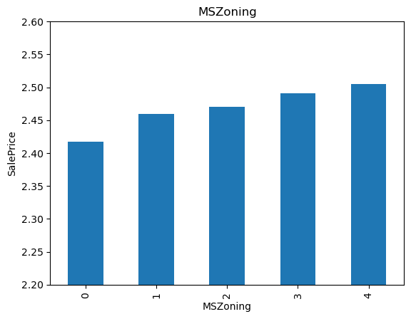
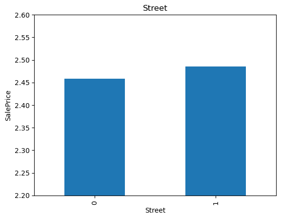
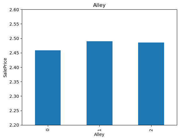
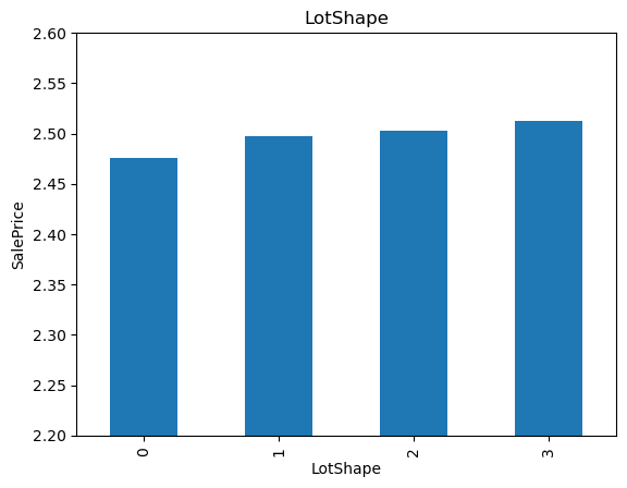
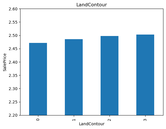
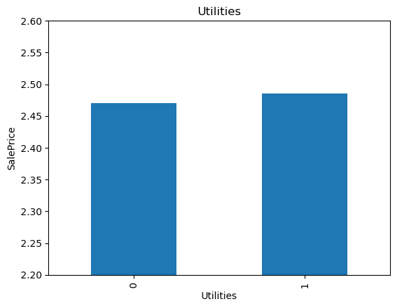
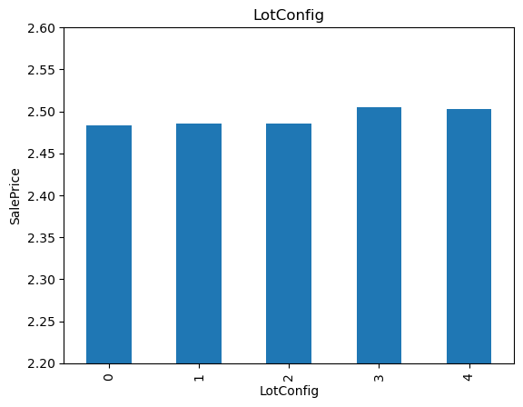
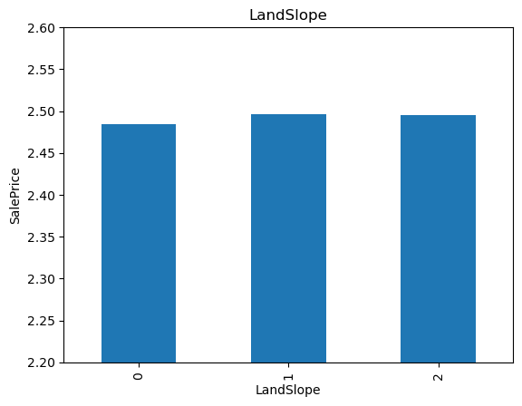
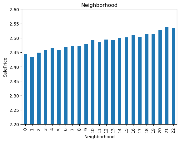
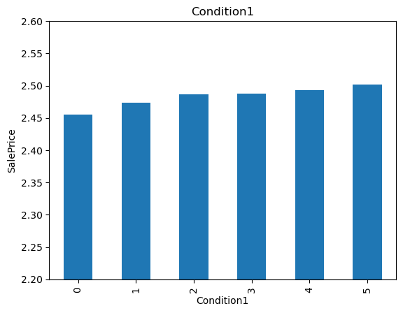
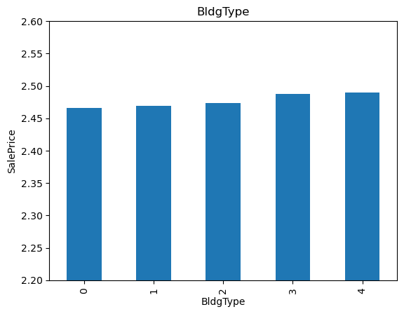
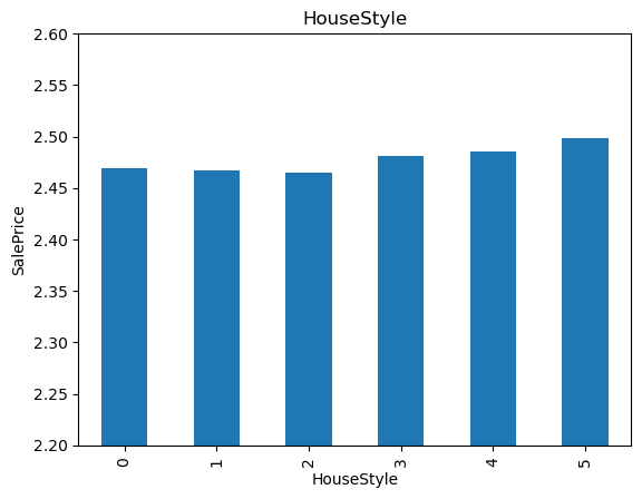
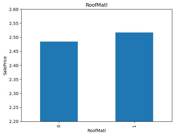
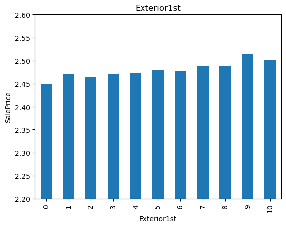
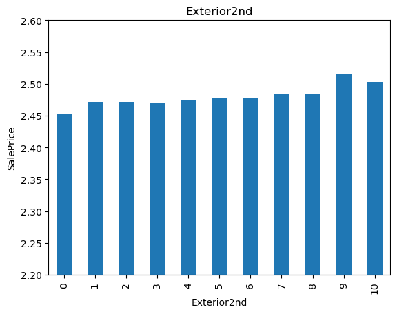
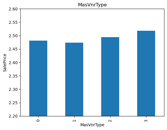
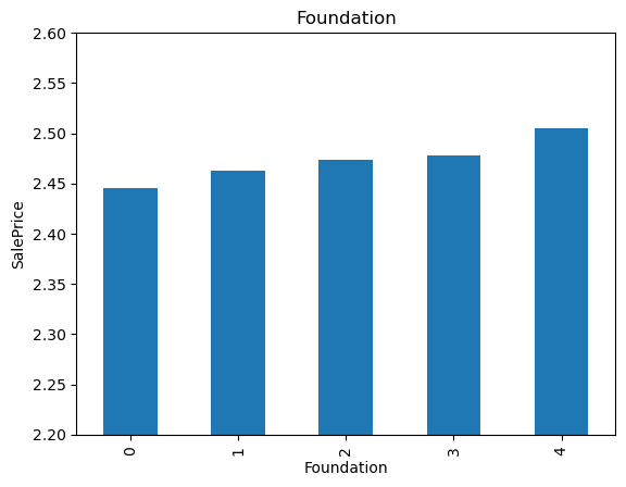
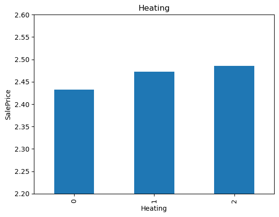
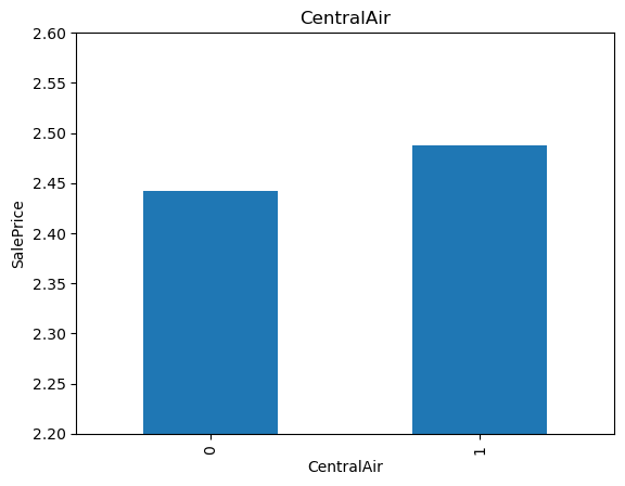
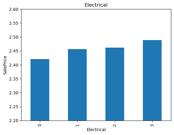
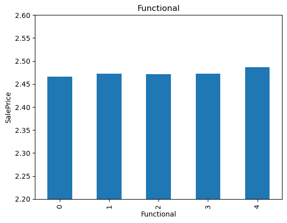
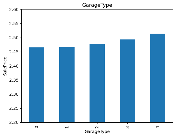
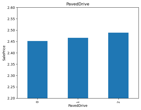
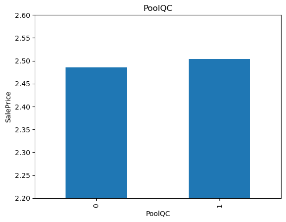
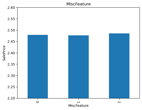
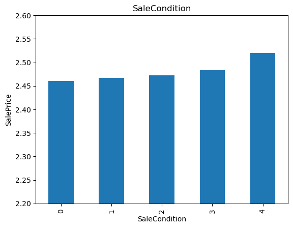
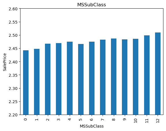
The monotonic relationship is particularly clear for the variables MSZoning and Neighborhood. Note how, the higher the integer that now represents the category, the higher the mean house sale price.

(The target is log-transformed, that is why the differences seem so small).

Feature Scaling

For use in linear models, features need to be scaled. Scaling features to the minimum and maximum values:

# create scaler
scaler = MinMaxScaler()

#  fit  the scaler to the train set
scaler.fit(X_train)

# transform the train and test set

# sklearn returns numpy arrays, so we wrap the
# array with a pandas dataframe

X_train = pd.DataFrame(scaler.transform(X_train), columns=X_train.columns)

X_test = pd.DataFrame(scaler.transform(X_test), columns=X_train.columns)

X_train.head()

	MSSubClass	MSZoning	LotFrontage	LotArea	Street	Alley	LotShape	LandContour	Utilities	LotConfig	LandSlope	Neighborhood	Condition1	Condition2	BldgType	HouseStyle	OverallQual	OverallCond	YearBuilt	YearRemodAdd	RoofStyle	RoofMatl	Exterior1st	Exterior2nd	MasVnrType	MasVnrArea	ExterQual	ExterCond	Foundation	BsmtQual	BsmtCond	BsmtExposure	BsmtFinType1	BsmtFinSF1	BsmtFinType2	BsmtFinSF2	BsmtUnfSF	TotalBsmtSF	Heating	HeatingQC	CentralAir	Electrical	1stFlrSF	2ndFlrSF	LowQualFinSF	GrLivArea	BsmtFullBath	BsmtHalfBath	FullBath	HalfBath	BedroomAbvGr	KitchenAbvGr	KitchenQual	TotRmsAbvGrd	Functional	Fireplaces	FireplaceQu	GarageType	GarageYrBlt	GarageFinish	GarageCars	GarageArea	GarageQual	GarageCond	PavedDrive	WoodDeckSF	OpenPorchSF	EnclosedPorch	3SsnPorch	ScreenPorch	PoolArea	PoolQC	Fence	MiscFeature	MiscVal	MoSold	SaleType	SaleCondition	LotFrontage_na	MasVnrArea_na	GarageYrBlt_na
0	0.750000	0.75	0.461171	0.366365	1.0	1.0	0.333333	1.000000	1.0	0.0	0.0	0.863636	0.4	1.0	0.75	0.6	0.777778	0.50	0.014706	0.049180	0.0	0.0	1.0	1.0	0.333333	0.00000	0.666667	0.5	1.0	0.666667	0.666667	0.666667	1.0	0.002835	0.0	0.0	0.673479	0.239935	1.0	1.00	1.0	1.0	0.559760	0.0	0.0	0.523250	0.000000	0.0	0.666667	0.0	0.375	0.333333	0.666667	0.416667	1.0	0.000000	0.0	0.75	0.018692	1.0	0.75	0.430183	0.5	0.5	1.0	0.116686	0.032907	0.0	0.0	0.0	0.0	0.0	0.00	1.0	0.0	0.545455	0.666667	0.75	0.0	0.0	0.0
1	0.750000	0.75	0.456066	0.388528	1.0	1.0	0.333333	0.333333	1.0	0.0	0.0	0.363636	0.4	1.0	0.75	0.6	0.444444	0.75	0.360294	0.049180	0.0	0.0	0.6	0.6	0.666667	0.03375	0.666667	0.5	0.5	0.333333	0.666667	0.000000	0.8	0.142807	0.0	0.0	0.114724	0.172340	1.0	1.00	1.0	1.0	0.434539	0.0	0.0	0.406196	0.333333	0.0	0.333333	0.5	0.375	0.333333	0.666667	0.250000	1.0	0.000000	0.0	0.75	0.457944	0.5	0.25	0.220028	0.5	0.5	1.0	0.000000	0.000000	0.0	0.0	0.0	0.0	0.0	0.75	1.0	0.0	0.636364	0.666667	0.75	0.0	0.0	0.0
2	0.916667	0.75	0.394699	0.336782	1.0	1.0	0.000000	0.333333	1.0	0.0	0.0	0.954545	0.4	1.0	1.00	0.6	0.888889	0.50	0.036765	0.098361	1.0	0.0	0.3	0.2	0.666667	0.25750	1.000000	0.5	1.0	1.000000	0.666667	0.000000	1.0	0.080794	0.0	0.0	0.601951	0.286743	1.0	1.00	1.0	1.0	0.627205	0.0	0.0	0.586296	0.333333	0.0	0.666667	0.0	0.250	0.333333	1.000000	0.333333	1.0	0.333333	0.8	0.75	0.046729	0.5	0.50	0.406206	0.5	0.5	1.0	0.228705	0.149909	0.0	0.0	0.0	0.0	0.0	0.00	1.0	0.0	0.090909	0.666667	0.75	0.0	0.0	0.0
3	0.750000	0.75	0.445002	0.482280	1.0	1.0	0.666667	0.666667	1.0	0.0	0.0	0.454545	0.4	1.0	0.75	0.6	0.666667	0.50	0.066176	0.163934	0.0	0.0	1.0	1.0	0.333333	0.00000	0.666667	0.5	1.0	0.666667	0.666667	1.000000	1.0	0.255670	0.0	0.0	0.018114	0.242553	1.0	1.00	1.0	1.0	0.566920	0.0	0.0	0.529943	0.333333	0.0	0.666667	0.0	0.375	0.333333	0.666667	0.250000	1.0	0.333333	0.4	0.75	0.084112	0.5	0.50	0.362482	0.5	0.5	1.0	0.469078	0.045704	0.0	0.0	0.0	0.0	0.0	0.00	1.0	0.0	0.636364	0.666667	0.75	1.0	0.0	0.0
4	0.750000	0.75	0.577658	0.391756	1.0	1.0	0.333333	0.333333	1.0	0.0	0.0	0.363636	0.4	1.0	0.75	0.6	0.555556	0.50	0.323529	0.737705	0.0	0.0	0.6	0.7	0.666667	0.17000	0.333333	0.5	0.5	0.333333	0.666667	0.000000	0.6	0.086818	0.0	0.0	0.434278	0.233224	1.0	0.75	1.0	1.0	0.549026	0.0	0.0	0.513216	0.000000	0.0	0.666667	0.0	0.375	0.333333	0.333333	0.416667	1.0	0.333333	0.8	0.75	0.411215	0.5	0.50	0.406206	0.5	0.5	1.0	0.000000	0.000000	0.0	1.0	0.0	0.0	0.0	0.00	1.0	0.0	0.545455	0.666667	0.75	0.0	0.0	0.0

Conclusion

We now have several classes with parameters learned from the training dataset, that we can store and retrieve at a later stage, so that when a colleague comes with new data, we are in a better position to score it faster.

Still:

• we would need to save each class

• then we could load each class

• and apply each transformation individually.

Which sounds like a lot of work.

The good news is, we can reduce the amount of work, if we set up all the transformations within a pipeline.

IMPORTANT

In order to set up the entire feature transformation within a pipeline, we still need to create a class that can be used within a pipeline to map the categorical variables with the arbitrary mappings, and also, to capture elapsed time between the temporal variables.