

Transportation costs and distance to work factors#
Two possible causes for absenteeism may also be the distance between home and work (the Distance from Residence to Work column) and transportation costs (the Transportation expense column). Employees who have to travel longer, or whose costs for commuting to work are high, might be more prone to absenteeism.
Importing libraries and packages#
 1# Mathematical operations and data manipulation
 2import pandas as pd
 3
 4# Statistics
 5from scipy.stats import yeojohnson
 6from scipy.stats import pearsonr
 7
 8# Plotting
 9import seaborn as sns
10import matplotlib.pyplot as plt
11
12# Warnings
13import warnings
14
15warnings.filterwarnings("ignore")
16
17%matplotlib inline
Set paths#
1# Path to datasets directory
2data_path = "./datasets"
3# Path to assets directory (for saving results to)
4assets_path = "./assets"
Loading dataset#
1# load data
2dataset = pd.read_csv(f"{data_path}/preprocessed_absenteism.csv")
3dataset.head()
| ID | Reason for absence | Month of absence | Day of the week | Seasons | Transportation expense | Distance from Residence to Work | Service time | Age | Work load Average/day | ... | Disciplinary failure | Education | Son | Social drinker | Social smoker | Pet | Weight | Height | Body mass index | Absenteeism time in hours | |
|---|---|---|---|---|---|---|---|---|---|---|---|---|---|---|---|---|---|---|---|---|---|
| 0 | 11 | 26 | July | Tuesday | Spring | 289 | 36 | 13 | 33 | 239.554 | ... | No | high_school | 2 | Yes | No | 1 | 90 | 172 | 30 | 4 |
| 1 | 36 | 0 | July | Tuesday | Spring | 118 | 13 | 18 | 50 | 239.554 | ... | Yes | high_school | 1 | Yes | No | 0 | 98 | 178 | 31 | 0 |
| 2 | 3 | 23 | July | Wednesday | Spring | 179 | 51 | 18 | 38 | 239.554 | ... | No | high_school | 0 | Yes | No | 0 | 89 | 170 | 31 | 2 |
| 3 | 7 | 7 | July | Thursday | Spring | 279 | 5 | 14 | 39 | 239.554 | ... | No | high_school | 2 | Yes | Yes | 0 | 68 | 168 | 24 | 4 |
| 4 | 11 | 23 | July | Thursday | Spring | 289 | 36 | 13 | 33 | 239.554 | ... | No | high_school | 2 | Yes | No | 1 | 90 | 172 | 30 | 2 |
5 rows × 21 columns
Exploring dataset#
1# Printing dimensionality of the data, columns, types and missing values
2print(f"Data dimension: {dataset.shape}")
3for col in dataset.columns:
4    print(
5        f"Column: {col:35} | "
6        f"type: {str(dataset[col].dtype):7} | "
7        f"missing values: {dataset[col].isna().sum():3d}"
8    )
Data dimension: (740, 21)
Column: ID                                  | type: int64   | missing values:   0
Column: Reason for absence                  | type: int64   | missing values:   0
Column: Month of absence                    | type: object  | missing values:   0
Column: Day of the week                     | type: object  | missing values:   0
Column: Seasons                             | type: object  | missing values:   0
Column: Transportation expense              | type: int64   | missing values:   0
Column: Distance from Residence to Work     | type: int64   | missing values:   0
Column: Service time                        | type: int64   | missing values:   0
Column: Age                                 | type: int64   | missing values:   0
Column: Work load Average/day               | type: float64 | missing values:   0
Column: Hit target                          | type: int64   | missing values:   0
Column: Disciplinary failure                | type: object  | missing values:   0
Column: Education                           | type: object  | missing values:   0
Column: Son                                 | type: int64   | missing values:   0
Column: Social drinker                      | type: object  | missing values:   0
Column: Social smoker                       | type: object  | missing values:   0
Column: Pet                                 | type: int64   | missing values:   0
Column: Weight                              | type: int64   | missing values:   0
Column: Height                              | type: int64   | missing values:   0
Column: Body mass index                     | type: int64   | missing values:   0
Column: Absenteeism time in hours           | type: int64   | missing values:   0
1# Computing statistics on numerical features
2dataset.describe().T
| count | mean | std | min | 25% | 50% | 75% | max | |
|---|---|---|---|---|---|---|---|---|
| ID | 740.0 | 18.017568 | 11.021247 | 1.000 | 9.000 | 18.000 | 28.000 | 36.000 |
| Reason for absence | 740.0 | 19.216216 | 8.433406 | 0.000 | 13.000 | 23.000 | 26.000 | 28.000 |
| Transportation expense | 740.0 | 221.329730 | 66.952223 | 118.000 | 179.000 | 225.000 | 260.000 | 388.000 |
| Distance from Residence to Work | 740.0 | 29.631081 | 14.836788 | 5.000 | 16.000 | 26.000 | 50.000 | 52.000 |
| Service time | 740.0 | 12.554054 | 4.384873 | 1.000 | 9.000 | 13.000 | 16.000 | 29.000 |
| Age | 740.0 | 36.450000 | 6.478772 | 27.000 | 31.000 | 37.000 | 40.000 | 58.000 |
| Work load Average/day | 740.0 | 271.490235 | 39.058116 | 205.917 | 244.387 | 264.249 | 294.217 | 378.884 |
| Hit target | 740.0 | 94.587838 | 3.779313 | 81.000 | 93.000 | 95.000 | 97.000 | 100.000 |
| Son | 740.0 | 1.018919 | 1.098489 | 0.000 | 0.000 | 1.000 | 2.000 | 4.000 |
| Pet | 740.0 | 0.745946 | 1.318258 | 0.000 | 0.000 | 0.000 | 1.000 | 8.000 |
| Weight | 740.0 | 79.035135 | 12.883211 | 56.000 | 69.000 | 83.000 | 89.000 | 108.000 |
| Height | 740.0 | 172.114865 | 6.034995 | 163.000 | 169.000 | 170.000 | 172.000 | 196.000 |
| Body mass index | 740.0 | 26.677027 | 4.285452 | 19.000 | 24.000 | 25.000 | 31.000 | 38.000 |
| Absenteeism time in hours | 740.0 | 6.924324 | 13.330998 | 0.000 | 2.000 | 3.000 | 8.000 | 120.000 |
Individual identification (ID)
Reason for absence (ICD). Absences attested by the International Code of Diseases (ICD) stratified into 21 categories (I to XXI) as follows:
I Certain infectious and parasitic diseases II Neoplasms III Diseases of the blood and blood-forming organs and certain disorders involving the immune mechanism IV Endocrine, nutritional and metabolic diseases V Mental and behavioural disorders VI Diseases of the nervous system VII Diseases of the eye and adnexa VIII Diseases of the ear and mastoid process IX Diseases of the circulatory system X Diseases of the respiratory system XI Diseases of the digestive system XII Diseases of the skin and subcutaneous tissue XIII Diseases of the musculoskeletal system and connective tissue XIV Diseases of the genitourinary system XV Pregnancy, childbirth and the puerperium XVI Certain conditions originating in the perinatal period XVII Congenital malformations, deformations and chromosomal abnormalities XVIII Symptoms, signs and abnormal clinical and laboratory findings, not elsewhere classified XIX Injury, poisoning and certain other consequences of external causes XX External causes of morbidity and mortality XXI Factors influencing health status and contact with health services.
And 7 categories without (CID) 2. patient follow-up (22), 3. medical consultation (23), 4. blood donation (24), 5. laboratory examination (25), 6. unjustified absence (26), 7. physiotherapy (27), 8. dental consultation (28).
Month of absence
Day of the week (Monday (2), Tuesday (3), Wednesday (4), Thursday (5), Friday (6))
Seasons (summer (1), autumn (2), winter (3), spring (4))
Transportation expense
Distance from Residence to Work (kilometers)
Service time
Age
Work load Average/day
Hit target
Disciplinary failure (yes=1; no=0)
Education (high school (1), graduate (2), postgraduate (3), master and doctor (4))
Son (number of children)
Social drinker (yes=1; no=0)
Social smoker (yes=1; no=0)
Pet (number of pet)
Weight
Height
Body mass index
Absenteeism time in hours (target)
Transportation costs and distance to work plots#
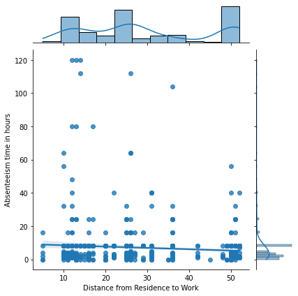
The seaborn jointplot() function not only produces the regression plot between the two variables but also estimates their distribution.
 1# Plotting transportation costs and distance to work agains hours
 2plt.figure(figsize=(10, 6))
 3sns.jointplot(
 4    x="Distance from Residence to Work",
 5    y="Absenteeism time in hours",
 6    data=dataset,
 7    kind="reg",
 8)
 9plt.savefig(f"{assets_path}/distance_vs_hours.png", format="png")
10
11plt.figure(figsize=(10, 6))
12sns.jointplot(
13    x="Transportation expense",
14    y="Absenteeism time in hours",
15    data=dataset,
16    kind="reg",
17)
18plt.savefig(f"{assets_path}/costs_vs_hours.png", format="png")
<Figure size 720x432 with 0 Axes>
<Figure size 720x432 with 0 Axes>
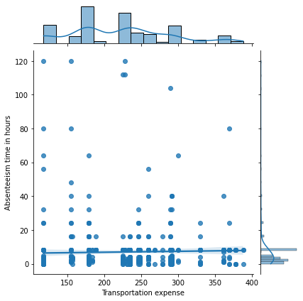
The distributions of Distance from Residence to Work and Transportation expense look close to normal distributions, while the absenteeism time in hours is heavily right-skewed. This makes the comparison between the variables difficult to interpret. One solution to this problem is to transform the data into something close to a normal distribution. A handy way to do this transformation is to use the Box-Cox or Yeo-Johnson transformations.
 1hours = yeojohnson(dataset["Absenteeism time in hours"].apply(float))
 2distances = dataset["Distance from Residence to Work"]
 3expenses = dataset["Transportation expense"]
 4
 5plt.figure(figsize=(10, 6))
 6ax = sns.jointplot(x=distances, y=hours[0], kind="reg")
 7ax.set_axis_labels(
 8    "Distance from Residence to Work", "Transformed absenteeism time in hours"
 9)
10plt.savefig(f"{assets_path}/distance_vs_hours_transformed.png", format="png")
11
12plt.figure(figsize=(10, 6))
13ax = sns.jointplot(x=expenses, y=hours[0], kind="reg")
14ax.set_axis_labels(
15    "Transportation expense", "Transformed absenteeism time in hours"
16)
17plt.savefig(f"{assets_path}/costs_vs_hours_transformed.png", format="png")
<Figure size 720x432 with 0 Axes>
<Figure size 720x432 with 0 Axes>
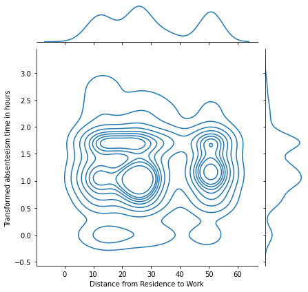
Producing kernel density estimation plots (that is, plots that help visualize the probability density functions of continuous variables) can be made by changing the type of the jointplot() function to kde.
 1# Producing KDE plots
 2
 3plt.figure(figsize=(10, 6))
 4ax = sns.jointplot(x=distances, y=hours[0], kind="kde")
 5ax.set_axis_labels(
 6    "Distance from Residence to Work", "Transformed absenteeism time in hours"
 7)
 8plt.savefig(
 9    f"{assets_path}/distance_vs_hours_transformed_kde.png", format="png"
10)
11
12plt.figure(figsize=(10, 6))
13ax = sns.jointplot(x=expenses, y=hours[0], kind="kde")
14ax.set_axis_labels(
15    "Transportation expense", "Transformed absenteeism time in hours"
16)
17plt.savefig(f"{assets_path}/costs_vs_hours_transformed_kde.png", format="png")
<Figure size 720x432 with 0 Axes>
<Figure size 720x432 with 0 Axes>
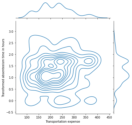
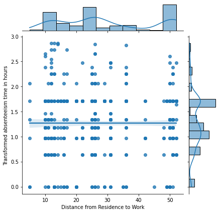
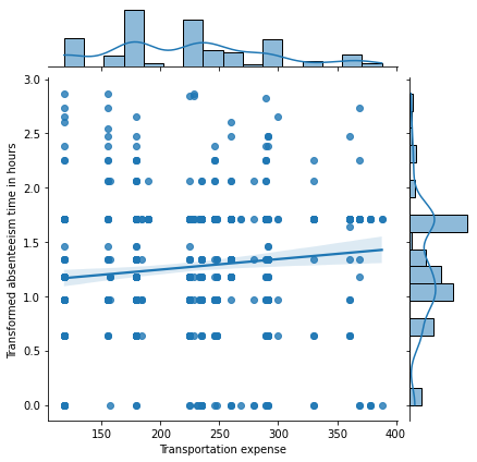
The regression line between the variables is almost flat for the Distance from Residence to Work column (which is a clear indicator of zero correlation) but has a slight upward slope for the Transportation Expense column. Therefore, we can expect a small positive correlation:
 1# Correlations between the columns
 2distance_corr = pearsonr(hours[0], distances)
 3expenses_corr = pearsonr(hours[0], expenses)
 4
 5print(
 6    f"Distances correlation: corr={distance_corr[0]:.3f}, "
 7    f"pvalue={distance_corr[1]:.3f}"
 8)
 9print(
10    f"Expenses comparison:  corr={expenses_corr[0]:.3f}, "
11    f"pvalue={expenses_corr[1]:.3f}"
12)
Distances correlation: corr=-0.000, pvalue=0.999
Expenses comparison:  corr=0.113, pvalue=0.002
These results confirm there is a slight positive correlation between Transportation expense and Absenteeism time in hours.