Data analysis

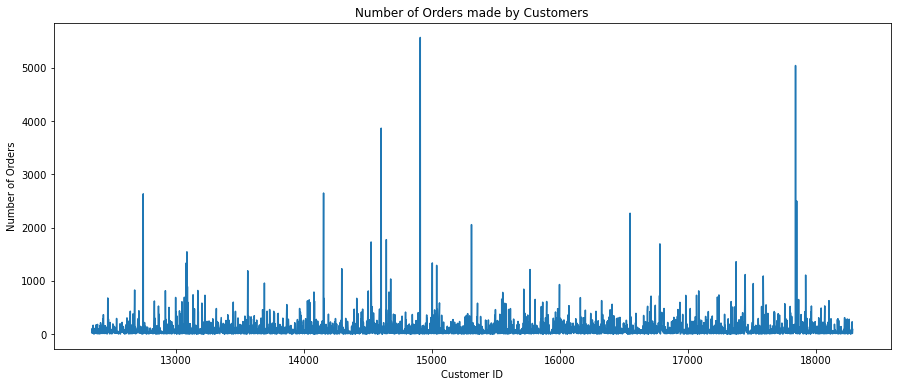
• Which customers placed the most and fewest orders?

• Which customers spent the most and least money?

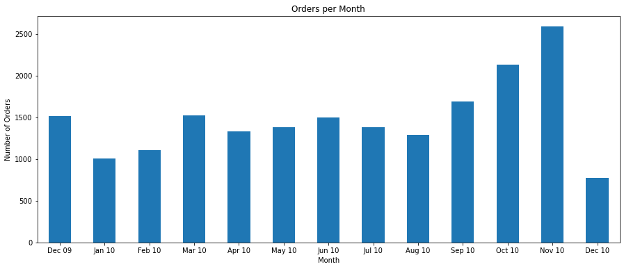
• Which months were the most and least popular for this online retail store?

• Which dates of the month were the most and least popular for this online retail store?

• Which days were the most and least popular for this online retail store?

• Which hours of the day were most and least popular for this online retail store?

• Which items were ordered the most and least?

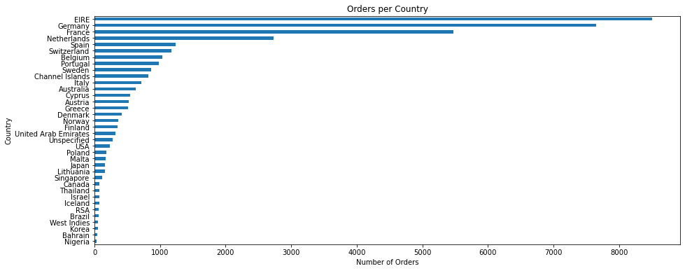
• Which countries placed the most and fewest orders?

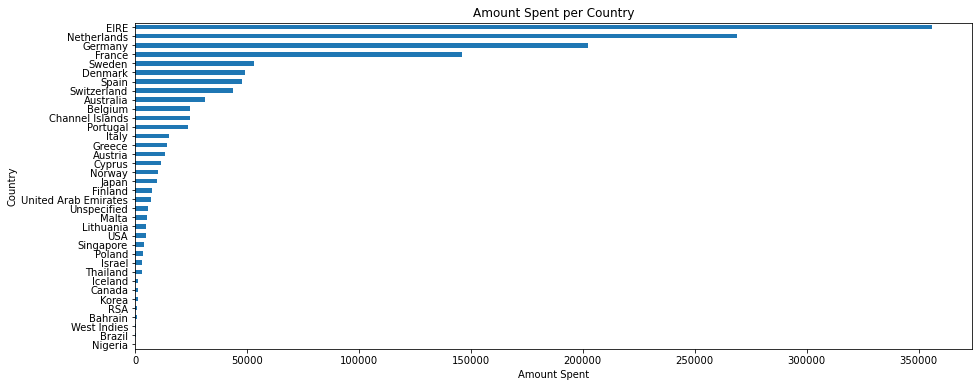
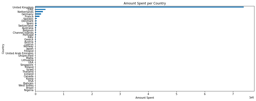
• Which countries spent the most and least money?

Importing libraries and packages

# Mathematical operations and data manipulation
import pandas as pd

# Visualisation
import matplotlib.pyplot as plt

# Warnings
import warnings

warnings.filterwarnings("ignore")

%matplotlib inline

Set paths

# Path to datasets directory
data_path = "./datasets"
# Path to assets directory (for saving results to)
assets_path = "./assets"

Loading dataset

# load data
dataset = pd.read_csv(f"{data_path}/engineered_retail.csv")
dataset.head().T

	0	1	2	3	4
invoice	489434	489434	489434	489434	489434
country	United Kingdom	United Kingdom	United Kingdom	United Kingdom	United Kingdom
cust_id	13085.0	13085.0	13085.0	13085.0	13085.0
stock_code	85048	79323P	79323W	22041	21232
desc	15cm christmas glass ball 20 lights	pink cherry lights	white cherry lights	record frame 7" single size	strawberry ceramic trinket box
quantity	12	12	12	48	24
unit_price	6.95	6.75	6.75	2.1	1.25
date	2009-12-01 07:45:00	2009-12-01 07:45:00	2009-12-01 07:45:00	2009-12-01 07:45:00	2009-12-01 07:45:00
spent	83.4	81.0	81.0	100.8	30.0
year_month	200912	200912	200912	200912	200912
year	2009	2009	2009	2009	2009
month	12	12	12	12	12
day	1	1	1	1	1
day_of_week	2	2	2	2	2
hour	7	7	7	7	7

Data analysis

Which customers placed the most and fewest orders?

# Orders by each customer
ord_cust = dataset.groupby(by=["cust_id", "country"], as_index=False)[
    "invoice"
].count()
ord_cust.head(10)

	cust_id	country	invoice
0	12346.0	United Kingdom	33
1	12347.0	Iceland	71
2	12348.0	Finland	20
3	12349.0	Italy	102
4	12351.0	Unspecified	21
5	12352.0	Norway	18
6	12353.0	Bahrain	20
7	12355.0	Bahrain	22
8	12356.0	Portugal	84
9	12357.0	Switzerland	165

plt.subplots(figsize=(15, 6))
oc = plt.plot(ord_cust.cust_id, ord_cust.invoice)
plt.xlabel("Customer ID")
plt.ylabel("Number of Orders")
plt.title("Number of Orders made by Customers")
plt.show()

# The top 5 customers
ord_cust.describe()

	cust_id	invoice
count	4315.000000	4315.000000
mean	15346.442642	94.474623
std	1702.986420	201.977000
min	12346.000000	1.000000
25%	13878.500000	18.000000
50%	15346.000000	44.000000
75%	16833.500000	102.000000
max	18287.000000	5570.000000

# 5 customers who ordered the most often
ord_cust.sort_values(by="invoice", ascending=False).head()

	cust_id	country	invoice
1844	14911.0	EIRE	5570
3992	17841.0	United Kingdom	5043
1610	14606.0	United Kingdom	3866
1273	14156.0	EIRE	2648
256	12748.0	United Kingdom	2633

# Who placed the fewest orders
ord_cust.sort_values(by="invoice", ascending=False).tail()

	cust_id	country	invoice
1233	14095.0	United Kingdom	1
1239	14106.0	United Kingdom	1
2752	16165.0	United Kingdom	1
3655	17378.0	United Kingdom	1
1427	14366.0	United Kingdom	1

Which customers spent the most and least money on an item?

spent_cust = dataset.groupby(
    by=["cust_id", "country", "quantity", "unit_price"], as_index=False
)["spent"].sum()
spent_cust.head()

	cust_id	country	quantity	unit_price	spent
0	12346.0	United Kingdom	1	1.00	1.00
1	12346.0	United Kingdom	1	3.25	3.25
2	12346.0	United Kingdom	1	5.95	23.80
3	12346.0	United Kingdom	1	7.49	142.31
4	12346.0	United Kingdom	5	4.50	157.50

plt.subplots(figsize=(15, 6))
sc = plt.plot(spent_cust.cust_id, spent_cust.spent)
plt.xlabel("Customer ID")
plt.ylabel("Total Amount Spent")
plt.title("Amount Spent by Customers")
plt.show()

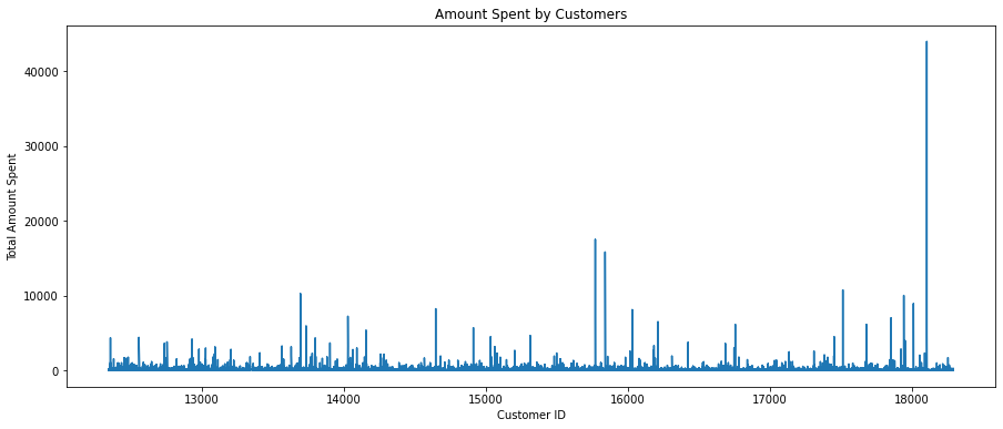
# Spent the most
spent_cust.sort_values(by="spent", ascending=False).head()

	cust_id	country	quantity	unit_price	spent
144871	18102.0	United Kingdom	300	4.58	43968.0
144915	18102.0	United Kingdom	600	3.00	18000.0
82744	15769.0	United Kingdom	200	1.65	17490.0
84312	15838.0	United Kingdom	9360	1.69	15818.4
144912	18102.0	United Kingdom	576	3.00	13824.0

# Spent the least
spent_cust.sort_values(by="spent", ascending=False).tail()

	cust_id	country	quantity	unit_price	spent
21568	13317.0	United Kingdom	1	0.001	0.001
61105	14857.0	United Kingdom	1	0.001	0.001
48967	14459.0	United Kingdom	1	0.001	0.001
6111	12671.0	Germany	1	0.001	0.001
32451	13765.0	United Kingdom	1	0.001	0.001

Which months were the most and least popular for this online retail store?

ord_month = (
    dataset.groupby(["invoice"])["year_month"]
    .unique()
    .value_counts()
    .sort_index()
)
ord_month

[200912]    1512
[201001]    1010
[201002]    1104
[201003]    1521
[201004]    1329
[201005]    1377
[201006]    1497
[201007]    1381
[201008]    1293
[201009]    1688
[201010]    2133
[201011]    2587
[201012]     776
Name: year_month, dtype: int64

om = ord_month.plot(kind="bar", figsize=(15, 6))
om.set_xlabel("Month")
om.set_ylabel("Number of Orders")
om.set_title("Orders per Month")
om.set_xticklabels(
    (
        "Dec 09",
        "Jan 10",
        "Feb 10",
        "Mar 10",
        "Apr 10",
        "May 10",
        "Jun 10",
        "Jul 10",
        "Aug 10",
        "Sep 10",
        "Oct 10",
        "Nov 10",
        "Dec 10",
    ),
    rotation="horizontal",
)
plt.show()

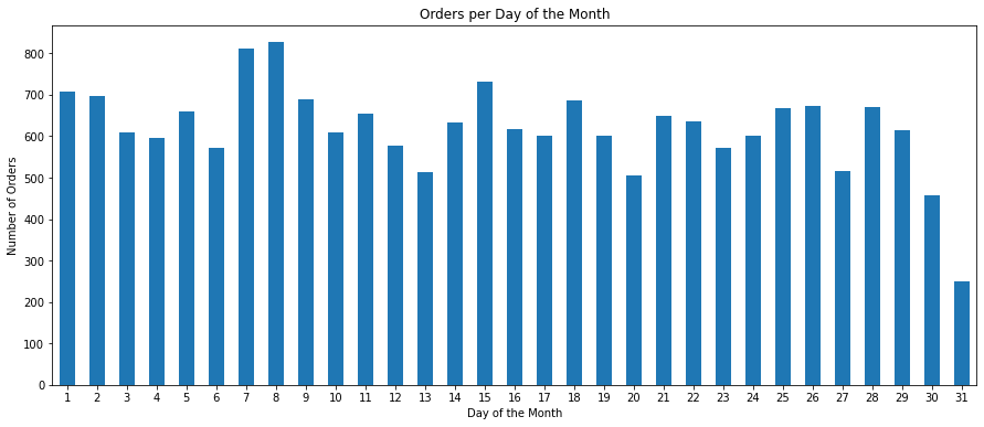
Which dates of the month were the most and least popular for this online retail store?

ord_day = (
    dataset.groupby("invoice")["day"].unique().value_counts().sort_index()
)
ord_day

[1]     708
[2]     696
[3]     610
[4]     595
[5]     661
[6]     572
[7]     812
[8]     827
[9]     689
[10]    609
[11]    655
[12]    576
[13]    512
[14]    634
[15]    732
[16]    617
[17]    600
[18]    687
[19]    601
[20]    506
[21]    649
[22]    636
[23]    573
[24]    602
[25]    667
[26]    672
[27]    517
[28]    671
[29]    614
[30]    457
[31]    251
Name: day, dtype: int64

od = ord_day.plot(kind="bar", figsize=(15, 6))
od.set_xlabel("Day of the Month")
od.set_ylabel("Number of Orders")
od.set_title("Orders per Day of the Month")
od.set_xticklabels(labels=[i for i in range(1, 32)], rotation="horizontal")
plt.show()

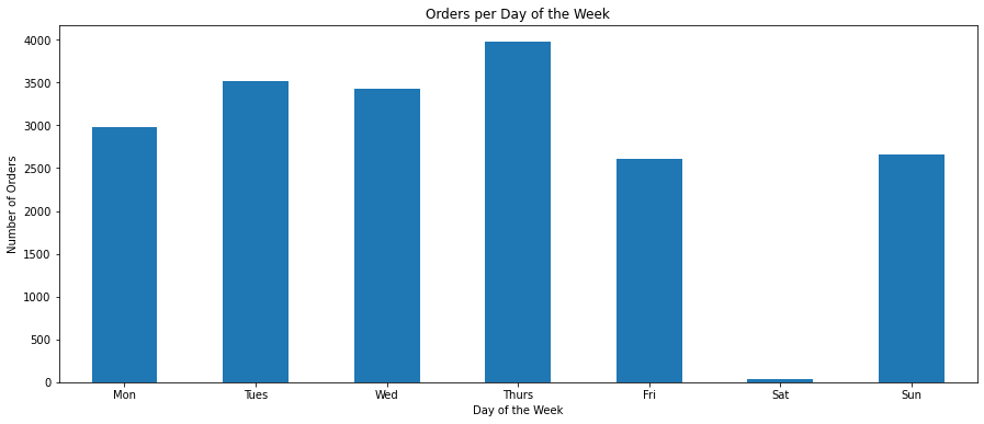
Which days were the most and least popular for this online retail store?

ord_dayofweek = (
    dataset.groupby("invoice")["day_of_week"]
    .unique()
    .value_counts()
    .sort_index()
)
ord_dayofweek

[1]    2985
[2]    3513
[3]    3426
[4]    3976
[5]    2612
[6]      30
[7]    2666
Name: day_of_week, dtype: int64

odw = ord_dayofweek.plot(kind="bar", figsize=(15, 6))
odw.set_xlabel("Day of the Week")
odw.set_ylabel("Number of Orders")
odw.set_title("Orders per Day of the Week")
odw.set_xticklabels(
    labels=["Mon", "Tues", "Wed", "Thurs", "Fri", "Sat", "Sun"],
    rotation="horizontal",
)
plt.show()

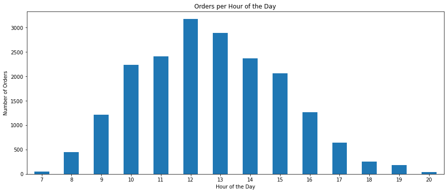
Which hours of the day were most and least popular for this online retail store?

ord_hour = (
    dataset.groupby(by=["invoice"])["hour"]
    .unique()
    .value_counts()
    .sort_index()
)
ord_hour

[7]       49
[8]      444
[9]     1209
[10]    2232
[11]    2407
[12]    3173
[13]    2891
[14]    2365
[15]    2061
[16]    1263
[17]     637
[18]     258
[19]     185
[20]      34
Name: hour, dtype: int64

oh = ord_hour.plot(kind="bar", figsize=(15, 6))
oh.set_xlabel("Hour of the Day")
oh.set_ylabel("Number of Orders")
oh.set_title("Orders per Hour of the Day")
oh.set_xticklabels(labels=[i for i in range(7, 21)], rotation="horizontal")
plt.show()

Which items were ordered the most and least?

q_item = dataset.groupby(by=["desc"], as_index=False)["quantity"].sum()
q_item.head()

	desc	quantity
0	doormat union jack guns and roses	169
1	3 stripey mice feltcraft	663
2	4 purple flock dinner candles	200
3	animal stickers	385
4	bank charges	2

q_item.sort_values(by="quantity", ascending=False).head()

	desc	quantity
4260	white hanging heart t-light holder	56915
4366	world war 2 gliders asstd designs	54754
691	brocade ring purse	48166
2632	pack of 72 retro spot cake cases	45156
262	assorted colour bird ornament	44551

q_item.sort_values(by="quantity", ascending=False).tail()

	desc	quantity
2544	opal white/silver flower necklace	1
1789	green chenille shaggy c/cover	1
2337	midnight blue crystal drop earrings	1
3728	silicon cube 25w, blue	1
1381	f.fairy s/3 sml candle, lavender	1

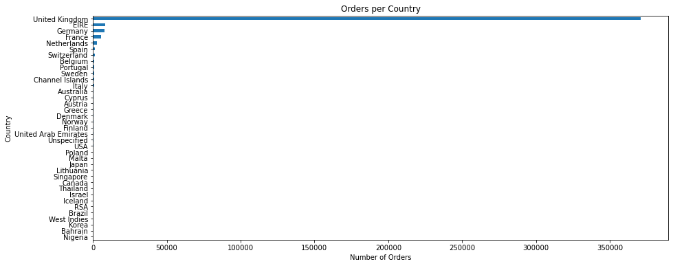
Which countries placed the most and fewest orders?

ord_coun = dataset.groupby(["country"])["invoice"].count().sort_values()
ord_coun.head()

country
Nigeria        30
Bahrain        42
Korea          53
West Indies    54
Brazil         62
Name: invoice, dtype: int64

ocoun = ord_coun.plot(kind="barh", figsize=(15, 6))
ocoun.set_xlabel("Number of Orders")
ocoun.set_ylabel("Country")
ocoun.set_title("Orders per Country")
plt.show()

del ord_coun["United Kingdom"]

ocoun2 = ord_coun.plot(kind="barh", figsize=(15, 6))
ocoun2.set_xlabel("Number of Orders")
ocoun2.set_ylabel("Country")
ocoun2.set_title("Orders per Country")
plt.show()

Which countries spent the most and least money?

coun_spent = dataset.groupby("country")["spent"].sum().sort_values()

cs = coun_spent.plot(kind="barh", figsize=(15, 6))
cs.set_xlabel("Amount Spent")
cs.set_ylabel("Country")
cs.set_title("Amount Spent per Country")
plt.show()

del coun_spent["United Kingdom"]

cs2 = coun_spent.plot(kind="barh", figsize=(15, 6))
cs2.set_xlabel("Amount Spent")
cs2.set_ylabel("Country")
cs2.set_title("Amount Spent per Country")
plt.show()