Analysis of weather related features#
Analysis of the group of features (weathersit, temp, atemp, hump and windspeed) representing the weather conditions. Expectation is to observe a strong dependency of those features on the current number of rides, as bad weather can significantly influence bike sharing services.
Importing libraries and packages#
 1# Mathematical operations and data manipulation
 2import numpy as np
 3import pandas as pd
 4from scipy.stats import pearsonr, spearmanr
 5
 6# Plotting
 7import seaborn as sns
 8import matplotlib.pyplot as plt
 9
10# Warnings
11import warnings
12
13warnings.filterwarnings("ignore")
14
15%matplotlib inline
Set paths#
1# Path to datasets directory
2data_path = "./datasets"
3# Path to assets directory (for saving results to)
4assets_path = "./assets"
Loading dataset#
1# load hourly data
2dataset = pd.read_csv(f"{data_path}/preprocessed_hour.csv")
3dataset.head()
| instant | dteday | season | yr | mnth | hr | holiday | weekday | workingday | weathersit | temp | atemp | hum | windspeed | casual | registered | cnt | |
|---|---|---|---|---|---|---|---|---|---|---|---|---|---|---|---|---|---|
| 0 | 1 | 2011-01-01 | winter | 2011 | 1 | 0 | 0 | Saturday | 0 | clear | 0.24 | 0.2879 | 81.0 | 0.0 | 3 | 13 | 16 |
| 1 | 2 | 2011-01-01 | winter | 2011 | 1 | 1 | 0 | Saturday | 0 | clear | 0.22 | 0.2727 | 80.0 | 0.0 | 8 | 32 | 40 |
| 2 | 3 | 2011-01-01 | winter | 2011 | 1 | 2 | 0 | Saturday | 0 | clear | 0.22 | 0.2727 | 80.0 | 0.0 | 5 | 27 | 32 |
| 3 | 4 | 2011-01-01 | winter | 2011 | 1 | 3 | 0 | Saturday | 0 | clear | 0.24 | 0.2879 | 75.0 | 0.0 | 3 | 10 | 13 |
| 4 | 5 | 2011-01-01 | winter | 2011 | 1 | 4 | 0 | Saturday | 0 | clear | 0.24 | 0.2879 | 75.0 | 0.0 | 0 | 1 | 1 |
1# print some generic statistics about the data
2print(f"Shape of data: {dataset.shape}")
3print(f"Number of missing values in the data: {dataset.isnull().sum().sum()}")
4
5# get statistics on the numerical columns
6dataset.describe().T
Shape of data: (17379, 17)
Number of missing values in the data: 0
| count | mean | std | min | 25% | 50% | 75% | max | |
|---|---|---|---|---|---|---|---|---|
| instant | 17379.0 | 8690.000000 | 5017.029500 | 1.00 | 4345.5000 | 8690.0000 | 13034.5000 | 17379.0000 |
| yr | 17379.0 | 2011.502561 | 0.500008 | 2011.00 | 2011.0000 | 2012.0000 | 2012.0000 | 2012.0000 |
| mnth | 17379.0 | 6.537775 | 3.438776 | 1.00 | 4.0000 | 7.0000 | 10.0000 | 12.0000 |
| hr | 17379.0 | 11.546752 | 6.914405 | 0.00 | 6.0000 | 12.0000 | 18.0000 | 23.0000 |
| holiday | 17379.0 | 0.028770 | 0.167165 | 0.00 | 0.0000 | 0.0000 | 0.0000 | 1.0000 |
| workingday | 17379.0 | 0.682721 | 0.465431 | 0.00 | 0.0000 | 1.0000 | 1.0000 | 1.0000 |
| temp | 17379.0 | 0.496987 | 0.192556 | 0.02 | 0.3400 | 0.5000 | 0.6600 | 1.0000 |
| atemp | 17379.0 | 0.475775 | 0.171850 | 0.00 | 0.3333 | 0.4848 | 0.6212 | 1.0000 |
| hum | 17379.0 | 62.722884 | 19.292983 | 0.00 | 48.0000 | 63.0000 | 78.0000 | 100.0000 |
| windspeed | 17379.0 | 12.736540 | 8.196795 | 0.00 | 7.0015 | 12.9980 | 16.9979 | 56.9969 |
| casual | 17379.0 | 35.676218 | 49.305030 | 0.00 | 4.0000 | 17.0000 | 48.0000 | 367.0000 |
| registered | 17379.0 | 153.786869 | 151.357286 | 0.00 | 34.0000 | 115.0000 | 220.0000 | 886.0000 |
| cnt | 17379.0 | 189.463088 | 181.387599 | 1.00 | 40.0000 | 142.0000 | 281.0000 | 977.0000 |
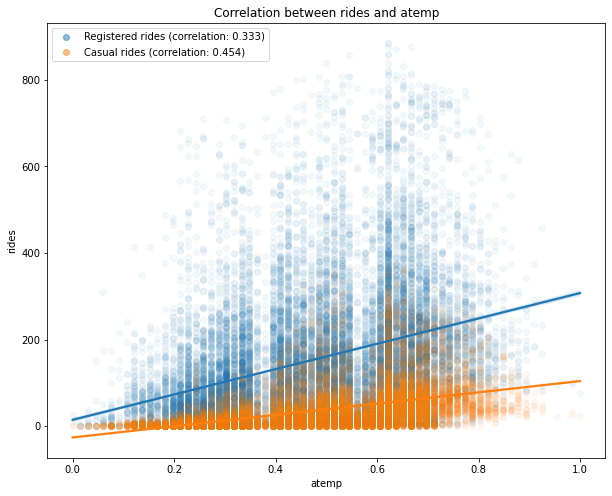
Correlation plots#
 1def plot_correlations(data, columns):
 2    # Correlation between col and registered rides
 3    corr_r = np.corrcoef(data[columns], data["registered"])[0, 1]
 4    sns.regplot(
 5        x=columns,
 6        y="registered",
 7        data=data,
 8        scatter_kws={"alpha": 0.05},
 9        label=f"Registered rides (correlation: {corr_r:.3f})",
10    )
11
12    # Correlation between col and casual rides
13    corr_c = np.corrcoef(data[columns], data["casual"])[0, 1]
14    ax = sns.regplot(
15        x=columns,
16        y="casual",
17        data=data,
18        scatter_kws={"alpha": 0.05},
19        label=f"Casual rides (correlation: {corr_c:.3f})",
20    )
21
22    # Adjusting legend alpha
23    legend = ax.legend()
24    for lh in legend.legendHandles:
25        lh.set_alpha(0.5)
26
27    ax.set_ylabel("rides")
28    ax.set_title(f"Correlation between rides and {columns}")
29    return ax
1plt.figure(figsize=(10, 8))
2ax = plot_correlations(dataset, "atemp")
3plt.savefig(f"{assets_path}/correlation_atemp.png", format="png")
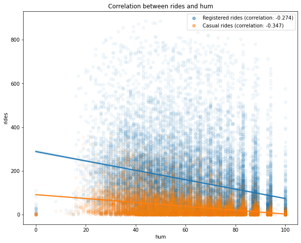
1plt.figure(figsize=(10, 8))
2ax = plot_correlations(dataset, "hum")
3plt.savefig(f"{assets_path}/correlation_hum.png", format="png")
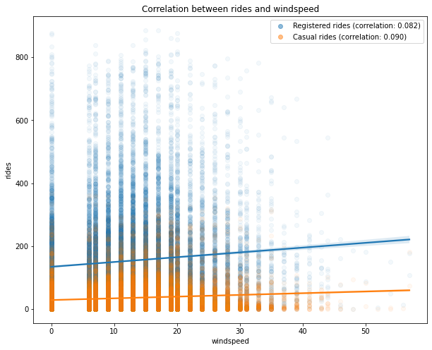
1plt.figure(figsize=(10, 8))
2ax = plot_correlations(dataset, "windspeed")
3plt.savefig(f"{assets_path}/correlation_windspeed.png", format="png")
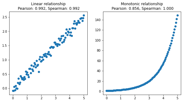
The difference between the Pearson and Spearman correlations#
 1# Random variables
 2x = np.linspace(0, 5, 100)
 3y_lin = 0.5 * x + 0.1 * np.random.randn(100)
 4y_mon = np.exp(x) + 0.1 * np.random.randn(100)
 5
 6# Correlations
 7corr_lin_pearson = pearsonr(x, y_lin)[0]
 8corr_lin_spearman = spearmanr(x, y_lin)[0]
 9corr_mon_pearson = pearsonr(x, y_mon)[0]
10corr_mon_spearman = spearmanr(x, y_mon)[0]
11
12# Visualizing variables
13fig, (ax1, ax2) = plt.subplots(1, 2, figsize=(10, 5))
14ax1.scatter(x, y_lin)
15ax1.set_title(
16    f"Linear relationship\n Pearson: {corr_lin_pearson:.3f}, "
17    f"Spearman: {corr_lin_spearman:.3f}"
18)
19ax2.scatter(x, y_mon)
20ax2.set_title(
21    f"Monotonic relationship\n Pearson: {corr_mon_pearson:.3f}, "
22    f"Spearman: {corr_mon_spearman:.3f}"
23)
24fig.savefig(f"{assets_path}/pearson_spearman.png", format="png")
 1# Function for computing correlations
 2def compute_correlations(data, columns):
 3    pearson_reg = pearsonr(data[columns], data["registered"])[0]
 4    pearson_cas = pearsonr(data[columns], data["casual"])[0]
 5    spearman_reg = spearmanr(data[columns], data["registered"])[0]
 6    spearman_cas = spearmanr(data[columns], data["casual"])[0]
 7
 8    return pd.Series(
 9        {
10            "Pearson (registered)": pearson_reg,
11            "Spearman (registered)": spearman_reg,
12            "Pearson (casual)": pearson_cas,
13            "Spearman (casual)": spearman_cas,
14        }
15    )
16
17
18# Correlation measures between different features
19cols = ["temp", "atemp", "hum", "windspeed"]
20corr_data = pd.DataFrame(
21    index=[
22        "Pearson (registered)",
23        "Spearman (registered)",
24        "Pearson (casual)",
25        "Spearman (casual)",
26    ]
27)
28
29for col in cols:
30    corr_data[col] = compute_correlations(dataset, col)
31
32corr_data.T
| Pearson (registered) | Spearman (registered) | Pearson (casual) | Spearman (casual) | |
|---|---|---|---|---|
| temp | 0.335361 | 0.373196 | 0.459616 | 0.570989 |
| atemp | 0.332559 | 0.373014 | 0.454080 | 0.570419 |
| hum | -0.273933 | -0.338480 | -0.347028 | -0.388213 |
| windspeed | 0.082321 | 0.122936 | 0.090287 | 0.122920 |
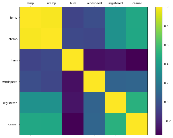
Correlation matrix#
 1# Plotting correlation matrix
 2cols = ["temp", "atemp", "hum", "windspeed", "registered", "casual"]
 3plot_data = dataset[cols]
 4corr = plot_data.corr()
 5
 6fig = plt.figure(figsize=(10, 8))
 7plt.matshow(corr, fignum=fig.number)
 8plt.xticks(range(len(plot_data.columns)), plot_data.columns)
 9plt.yticks(range(len(plot_data.columns)), plot_data.columns)
10plt.colorbar()
11plt.ylim([5.5, -0.5])
12fig.savefig(f"{assets_path}/correlation_matrix.png", format="png")