

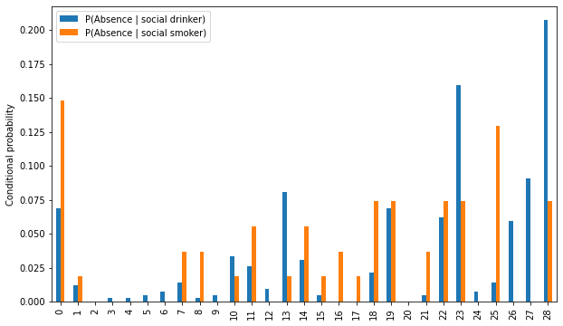
Conditional probabilities of the different absence reasons#
Computing the conditional probabilities of the different reasons for absence, assuming that the employee is a social drinker or smoker.
Importing libraries and packages#
 1# Mathematical operations and data manipulation
 2import pandas as pd
 3
 4# Statistics
 5from scipy.stats import ttest_ind
 6from scipy.stats import ks_2samp
 7
 8# Plotting
 9import seaborn as sns
10import matplotlib.pyplot as plt
11
12# Warnings
13import warnings
14
15warnings.filterwarnings("ignore")
16
17%matplotlib inline
Set paths#
1# Path to datasets directory
2data_path = "./datasets"
3# Path to assets directory (for saving results to)
4assets_path = "./assets"
Loading dataset#
1# load data
2dataset = pd.read_csv(f"{data_path}/preprocessed_absenteism.csv")
3dataset.head()
| ID | Reason for absence | Month of absence | Day of the week | Seasons | Transportation expense | Distance from Residence to Work | Service time | Age | Work load Average/day | ... | Disciplinary failure | Education | Son | Social drinker | Social smoker | Pet | Weight | Height | Body mass index | Absenteeism time in hours | |
|---|---|---|---|---|---|---|---|---|---|---|---|---|---|---|---|---|---|---|---|---|---|
| 0 | 11 | 26 | July | Tuesday | Spring | 289 | 36 | 13 | 33 | 239.554 | ... | No | high_school | 2 | Yes | No | 1 | 90 | 172 | 30 | 4 |
| 1 | 36 | 0 | July | Tuesday | Spring | 118 | 13 | 18 | 50 | 239.554 | ... | Yes | high_school | 1 | Yes | No | 0 | 98 | 178 | 31 | 0 |
| 2 | 3 | 23 | July | Wednesday | Spring | 179 | 51 | 18 | 38 | 239.554 | ... | No | high_school | 0 | Yes | No | 0 | 89 | 170 | 31 | 2 |
| 3 | 7 | 7 | July | Thursday | Spring | 279 | 5 | 14 | 39 | 239.554 | ... | No | high_school | 2 | Yes | Yes | 0 | 68 | 168 | 24 | 4 |
| 4 | 11 | 23 | July | Thursday | Spring | 289 | 36 | 13 | 33 | 239.554 | ... | No | high_school | 2 | Yes | No | 1 | 90 | 172 | 30 | 2 |
5 rows × 21 columns
Exploring dataset#
1# Printing dimensionality of the data, columns, types and missing values
2print(f"Data dimension: {dataset.shape}")
3for col in dataset.columns:
4    print(
5        f"Column: {col:35} | "
6        f"type: {str(dataset[col].dtype):7} | "
7        f"missing values: {dataset[col].isna().sum():3d}"
8    )
Data dimension: (740, 21)
Column: ID                                  | type: int64   | missing values:   0
Column: Reason for absence                  | type: int64   | missing values:   0
Column: Month of absence                    | type: object  | missing values:   0
Column: Day of the week                     | type: object  | missing values:   0
Column: Seasons                             | type: object  | missing values:   0
Column: Transportation expense              | type: int64   | missing values:   0
Column: Distance from Residence to Work     | type: int64   | missing values:   0
Column: Service time                        | type: int64   | missing values:   0
Column: Age                                 | type: int64   | missing values:   0
Column: Work load Average/day               | type: float64 | missing values:   0
Column: Hit target                          | type: int64   | missing values:   0
Column: Disciplinary failure                | type: object  | missing values:   0
Column: Education                           | type: object  | missing values:   0
Column: Son                                 | type: int64   | missing values:   0
Column: Social drinker                      | type: object  | missing values:   0
Column: Social smoker                       | type: object  | missing values:   0
Column: Pet                                 | type: int64   | missing values:   0
Column: Weight                              | type: int64   | missing values:   0
Column: Height                              | type: int64   | missing values:   0
Column: Body mass index                     | type: int64   | missing values:   0
Column: Absenteeism time in hours           | type: int64   | missing values:   0
1# Computing statistics on numerical features
2dataset.describe().T
| count | mean | std | min | 25% | 50% | 75% | max | |
|---|---|---|---|---|---|---|---|---|
| ID | 740.0 | 18.017568 | 11.021247 | 1.000 | 9.000 | 18.000 | 28.000 | 36.000 |
| Reason for absence | 740.0 | 19.216216 | 8.433406 | 0.000 | 13.000 | 23.000 | 26.000 | 28.000 |
| Transportation expense | 740.0 | 221.329730 | 66.952223 | 118.000 | 179.000 | 225.000 | 260.000 | 388.000 |
| Distance from Residence to Work | 740.0 | 29.631081 | 14.836788 | 5.000 | 16.000 | 26.000 | 50.000 | 52.000 |
| Service time | 740.0 | 12.554054 | 4.384873 | 1.000 | 9.000 | 13.000 | 16.000 | 29.000 |
| Age | 740.0 | 36.450000 | 6.478772 | 27.000 | 31.000 | 37.000 | 40.000 | 58.000 |
| Work load Average/day | 740.0 | 271.490235 | 39.058116 | 205.917 | 244.387 | 264.249 | 294.217 | 378.884 |
| Hit target | 740.0 | 94.587838 | 3.779313 | 81.000 | 93.000 | 95.000 | 97.000 | 100.000 |
| Son | 740.0 | 1.018919 | 1.098489 | 0.000 | 0.000 | 1.000 | 2.000 | 4.000 |
| Pet | 740.0 | 0.745946 | 1.318258 | 0.000 | 0.000 | 0.000 | 1.000 | 8.000 |
| Weight | 740.0 | 79.035135 | 12.883211 | 56.000 | 69.000 | 83.000 | 89.000 | 108.000 |
| Height | 740.0 | 172.114865 | 6.034995 | 163.000 | 169.000 | 170.000 | 172.000 | 196.000 |
| Body mass index | 740.0 | 26.677027 | 4.285452 | 19.000 | 24.000 | 25.000 | 31.000 | 38.000 |
| Absenteeism time in hours | 740.0 | 6.924324 | 13.330998 | 0.000 | 2.000 | 3.000 | 8.000 | 120.000 |
Individual identification (ID)
Reason for absence (ICD). Absences attested by the International Code of Diseases (ICD) stratified into 21 categories (I to XXI) as follows:
I Certain infectious and parasitic diseases II Neoplasms III Diseases of the blood and blood-forming organs and certain disorders involving the immune mechanism IV Endocrine, nutritional and metabolic diseases V Mental and behavioural disorders VI Diseases of the nervous system VII Diseases of the eye and adnexa VIII Diseases of the ear and mastoid process IX Diseases of the circulatory system X Diseases of the respiratory system XI Diseases of the digestive system XII Diseases of the skin and subcutaneous tissue XIII Diseases of the musculoskeletal system and connective tissue XIV Diseases of the genitourinary system XV Pregnancy, childbirth and the puerperium XVI Certain conditions originating in the perinatal period XVII Congenital malformations, deformations and chromosomal abnormalities XVIII Symptoms, signs and abnormal clinical and laboratory findings, not elsewhere classified XIX Injury, poisoning and certain other consequences of external causes XX External causes of morbidity and mortality XXI Factors influencing health status and contact with health services.
And 7 categories without (CID) 2. patient follow-up (22), 3. medical consultation (23), 4. blood donation (24), 5. laboratory examination (25), 6. unjustified absence (26), 7. physiotherapy (27), 8. dental consultation (28).
Month of absence
Day of the week (Monday (2), Tuesday (3), Wednesday (4), Thursday (5), Friday (6))
Seasons (summer (1), autumn (2), winter (3), spring (4))
Transportation expense
Distance from Residence to Work (kilometers)
Service time
Age
Work load Average/day
Hit target
Disciplinary failure (yes=1; no=0)
Education (high school (1), graduate (2), postgraduate (3), master and doctor (4))
Son (number of children)
Social drinker (yes=1; no=0)
Social smoker (yes=1; no=0)
Pet (number of pet)
Weight
Height
Body mass index
Absenteeism time in hours (target)
Probabilities#
 1# Probabilities of being a drinker and smoker
 2drinker_prob = dataset["Social drinker"].value_counts(normalize=True)["Yes"]
 3smoker_prob = dataset["Social smoker"].value_counts(normalize=True)["Yes"]
 4print(
 5    f"P(social drinker) = {drinker_prob:.3f} | "
 6    f"P(social smoker) = {smoker_prob:.3f}"
 7)
 8
 9# Masks for social drinkers/smokers
10drinker_mask = dataset["Social drinker"] == "Yes"
11smoker_mask = dataset["Social smoker"] == "Yes"
12
13# Computing probabilities of absence reasons and being a social drinker/smoker
14total_entries = dataset.shape[0]
15absence_drinker_prob = (
16    dataset["Reason for absence"][drinker_mask].value_counts() / total_entries
17)
18absence_smoker_prob = (
19    dataset["Reason for absence"][smoker_mask].value_counts() / total_entries
20)
21
22# Computing conditional probabilities
23cond_prob = pd.DataFrame(index=range(0, 29))
24cond_prob["P(Absence | social drinker)"] = absence_drinker_prob / drinker_prob
25cond_prob["P(Absence | social smoker)"] = absence_smoker_prob / smoker_prob
26
27# Plotting probabilities
28plt.figure()
29ax = cond_prob.plot.bar(figsize=(10, 6))
30ax.set_ylabel("Conditional probability")
31plt.savefig(
32    f"{assets_path}/conditional_probabilities.png", format="png", dpi=300
33)
P(social drinker) = 0.568 | P(social smoker) = 0.073
<Figure size 432x288 with 0 Axes>
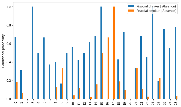
The probability of being a Drinker/Smoker, conditioned to absence reason#
1# Computing reason for absence probabilities
2absence_prob = dataset["Reason for absence"].value_counts(normalize=True)
 1# Computing conditional probabilities for drinker/smoker
 2cond_prob_drinker_smoker = pd.DataFrame(index=range(0, 29))
 3cond_prob_drinker_smoker["P(social drinker | Absence)"] = (
 4    cond_prob["P(Absence | social drinker)"] * drinker_prob / absence_prob
 5)
 6cond_prob_drinker_smoker["P(social smoker | Absence)"] = (
 7    cond_prob["P(Absence | social smoker)"] * smoker_prob / absence_prob
 8)
 9
10plt.figure()
11ax = cond_prob_drinker_smoker.plot.bar(figsize=(10, 6))
12ax.set_ylabel("Conditional probability")
13plt.savefig(
14    f"{assets_path}/conditional_probabilities_drinker_smoker.png",
15    format="png",
16    dpi=300,
17)
<Figure size 432x288 with 0 Axes>
 1# Creating violin plots of the absenteeism time in hours
 2plt.figure(figsize=(8, 6))
 3sns.violinplot(
 4    x="Social drinker",
 5    y="Absenteeism time in hours",
 6    data=dataset,
 7    order=["No", "Yes"],
 8)
 9plt.savefig(
10    f"{assets_path}/drinkers_hour_distribution.png", format="png", dpi=300
11)
12
13plt.figure(figsize=(8, 6))
14sns.violinplot(
15    x="Social smoker",
16    y="Absenteeism time in hours",
17    data=dataset,
18    order=["No", "Yes"],
19)
20plt.savefig(
21    f"{assets_path}/smokers_hour_distribution.png", format="png", dpi=300
22)
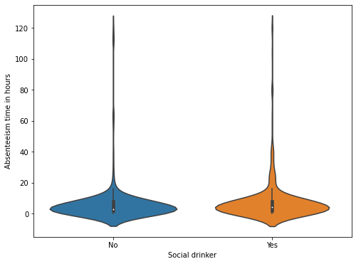
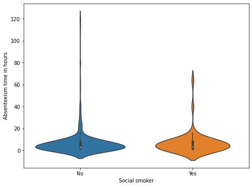
There seems to be no substantial difference in the distribution of absenteeism hours in drinkers and smokers.
Hypothesis testing#
Hypothesis testing on the absenteeism hours (with a null hypothesis stating that the average absenteeism time in hours is the same for drinkers and non-drinkers).
 1hours_col = "Absenteeism time in hours"
 2
 3# test mean absenteeism time for drinkers
 4drinkers_mask = dataset["Social drinker"] == "Yes"
 5hours_drinkers = dataset.loc[drinker_mask, hours_col]
 6hours_non_drinkers = dataset.loc[~drinker_mask, hours_col]
 7drinkers_test = ttest_ind(hours_drinkers, hours_non_drinkers)
 8print(f"Statistic value: {drinkers_test[0]}, p-value: {drinkers_test[1]}")
 9
10# test mean absenteeism time for smokers
11smokers_mask = dataset["Social smoker"] == "Yes"
12hours_smokers = dataset.loc[smokers_mask, hours_col]
13hours_non_smokers = dataset.loc[~smokers_mask, hours_col]
14smokers_test = ttest_ind(hours_smokers, hours_non_smokers)
15print(f"Statistic value: {smokers_test[0]}, p-value: {smokers_test[1]}")
Statistic value: 1.7713833295243993, p-value: 0.07690961828294651
Statistic value: -0.24277795417700243, p-value: 0.8082448720154971
The p-value of both tests is above the critical value of 0.05, which means the null hypothesis can not be rejected.
Kolmogorov-Smirnov test for comparing the distributions
 1ks_drinkers = ks_2samp(hours_drinkers, hours_non_drinkers)
 2ks_smokers = ks_2samp(hours_smokers, hours_non_smokers)
 3
 4print(
 5    f"Drinkers comparison: statistics={ks_drinkers[0]:.3f}, "
 6    f"pvalue={ks_drinkers[1]:.3f}"
 7)
 8print(
 9    f"Smokers comparison:  statistics={ks_smokers[0]:.3f}, "
10    f"pvalue={ks_smokers[1]:.3f}"
11)
Drinkers comparison: statistics=0.135, pvalue=0.002
Smokers comparison:  statistics=0.104, pvalue=0.607
The pvalue for the drinkers is much lower than the critical 0.05, strong evidence against the null hypothesis of the two distributions being equal.