

Regressions#
Loading the data and performing some initial exploration on it to acquire some basic knowledge about the data, how the various features are distributed.
Importing libraries and packages#
 1# Warnings
 2import warnings
 3
 4# Mathematical operations and data manipulation
 5import numpy as np
 6import pandas as pd
 7
 8# Statistics
 9import statsmodels.api as sm
10
11# Plotting
12import seaborn as sns
13import matplotlib.pyplot as plt
14
15warnings.filterwarnings("ignore")
16%matplotlib inline
---------------------------------------------------------------------------
ImportError                               Traceback (most recent call last)
Input In [1], in <cell line: 9>()
      6 import pandas as pd
      8 # Statistics
----> 9 import statsmodels.api as sm
     11 # Plotting
     12 import seaborn as sns

File ~/checkouts/readthedocs.org/user_builds/analysing/conda/latest/lib/python3.9/site-packages/statsmodels/api.py:105, in <module>
     94 from .genmod import api as genmod
     95 from .genmod.api import (
     96     GEE,
     97     GLM,
   (...)
    103     families,
    104 )
--> 105 from .graphics import api as graphics
    106 from .graphics.gofplots import ProbPlot, qqline, qqplot, qqplot_2samples
    107 from .imputation.bayes_mi import MI, BayesGaussMI

File ~/checkouts/readthedocs.org/user_builds/analysing/conda/latest/lib/python3.9/site-packages/statsmodels/graphics/api.py:1, in <module>
----> 1 from . import tsaplots as tsa
      2 from .agreement import mean_diff_plot
      3 from .boxplots import beanplot, violinplot

File ~/checkouts/readthedocs.org/user_builds/analysing/conda/latest/lib/python3.9/site-packages/statsmodels/graphics/tsaplots.py:11, in <module>
      8 import pandas as pd
     10 from statsmodels.graphics import utils
---> 11 from statsmodels.tsa.stattools import acf, pacf
     14 def _prepare_data_corr_plot(x, lags, zero):
     15     zero = bool(zero)

File ~/checkouts/readthedocs.org/user_builds/analysing/conda/latest/lib/python3.9/site-packages/statsmodels/tsa/stattools.py:19, in <module>
     17 from scipy import stats
     18 from scipy.interpolate import interp1d
---> 19 from scipy.signal import correlate
     21 from statsmodels.regression.linear_model import OLS, yule_walker
     22 from statsmodels.tools.sm_exceptions import (
     23     CollinearityWarning,
     24     InfeasibleTestError,
     25     InterpolationWarning,
     26     MissingDataError,
     27 )

File ~/checkouts/readthedocs.org/user_builds/analysing/conda/latest/lib/python3.9/site-packages/scipy/signal/__init__.py:309, in <module>
      1 """
      2 =======================================
      3 Signal processing (:mod:`scipy.signal`)
   (...)
    307
    308 """
--> 309 from . import _sigtools, windows
    310 from ._waveforms import *
    311 from ._max_len_seq import max_len_seq

File ~/checkouts/readthedocs.org/user_builds/analysing/conda/latest/lib/python3.9/site-packages/scipy/signal/windows/__init__.py:41, in <module>
      1 """
      2 Window functions (:mod:`scipy.signal.windows`)
      3 ==============================================
   (...)
     38
     39 """
---> 41 from ._windows import *
     43 # Deprecated namespaces, to be removed in v2.0.0
     44 from . import windows

File ~/checkouts/readthedocs.org/user_builds/analysing/conda/latest/lib/python3.9/site-packages/scipy/signal/windows/_windows.py:7, in <module>
      4 import warnings
      6 import numpy as np
----> 7 from scipy import linalg, special, fft as sp_fft
      9 __all__ = ['boxcar', 'triang', 'parzen', 'bohman', 'blackman', 'nuttall',
     10            'blackmanharris', 'flattop', 'bartlett', 'hanning', 'barthann',
     11            'hamming', 'kaiser', 'gaussian', 'general_cosine',
     12            'general_gaussian', 'general_hamming', 'chebwin', 'cosine',
     13            'hann', 'exponential', 'tukey', 'taylor', 'dpss', 'get_window']
     16 def _len_guards(M):

File ~/checkouts/readthedocs.org/user_builds/analysing/conda/latest/lib/python3.9/site-packages/scipy/fft/__init__.py:91, in <module>
     89 from ._realtransforms import dct, idct, dst, idst, dctn, idctn, dstn, idstn
     90 from ._fftlog import fht, ifht, fhtoffset
---> 91 from ._helper import next_fast_len
     92 from ._backend import (set_backend, skip_backend, set_global_backend,
     93                        register_backend)
     94 from numpy.fft import fftfreq, rfftfreq, fftshift, ifftshift

File ~/checkouts/readthedocs.org/user_builds/analysing/conda/latest/lib/python3.9/site-packages/scipy/fft/_helper.py:3, in <module>
      1 from functools import update_wrapper, lru_cache
----> 3 from ._pocketfft import helper as _helper
      6 def next_fast_len(target, real=False):
      7     """Find the next fast size of input data to ``fft``, for zero-padding, etc.
      8
      9     SciPy's FFT algorithms gain their speed by a recursive divide and conquer
   (...)
     59
     60     """

File ~/checkouts/readthedocs.org/user_builds/analysing/conda/latest/lib/python3.9/site-packages/scipy/fft/_pocketfft/__init__.py:3, in <module>
      1 """ FFT backend using pypocketfft """
----> 3 from .basic import *
      4 from .realtransforms import *
      5 from .helper import *

File ~/checkouts/readthedocs.org/user_builds/analysing/conda/latest/lib/python3.9/site-packages/scipy/fft/_pocketfft/basic.py:6, in <module>
      4 import numpy as np
      5 import functools
----> 6 from . import pypocketfft as pfft
      7 from .helper import (_asfarray, _init_nd_shape_and_axes, _datacopied,
      8                      _fix_shape, _fix_shape_1d, _normalization,
      9                      _workers)
     11 def c2c(forward, x, n=None, axis=-1, norm=None, overwrite_x=False,
     12         workers=None, *, plan=None):

ImportError: /home/docs/checkouts/readthedocs.org/user_builds/analysing/conda/latest/lib/python3.9/site-packages/zmq/backend/cython/../../../../.././libstdc++.so.6: version `GLIBCXX_3.4.30' not found (required by /home/docs/checkouts/readthedocs.org/user_builds/analysing/conda/latest/lib/python3.9/site-packages/scipy/fft/_pocketfft/pypocketfft.cpython-39-x86_64-linux-gnu.so)
Set paths#
1# Path to datasets directory
2data_path = "./datasets"
3# Path to assets directory (for saving results to)
4assets_path = "./assets"
Loading dataset#
1# load data
2dataset = pd.read_csv(f"{data_path}/bank-additional-full.csv", sep=";")
3dataset.head().T
| 0 | 1 | 2 | 3 | 4 | |
|---|---|---|---|---|---|
| age | 56 | 57 | 37 | 40 | 56 |
| job | housemaid | services | services | admin. | services |
| marital | married | married | married | married | married |
| education | basic.4y | high.school | high.school | basic.6y | high.school |
| default | no | unknown | no | no | no |
| housing | no | no | yes | no | no |
| loan | no | no | no | no | yes |
| contact | telephone | telephone | telephone | telephone | telephone |
| month | may | may | may | may | may |
| day_of_week | mon | mon | mon | mon | mon |
| duration | 261 | 149 | 226 | 151 | 307 |
| campaign | 1 | 1 | 1 | 1 | 1 |
| pdays | 999 | 999 | 999 | 999 | 999 |
| previous | 0 | 0 | 0 | 0 | 0 |
| poutcome | nonexistent | nonexistent | nonexistent | nonexistent | nonexistent |
| emp.var.rate | 1.1 | 1.1 | 1.1 | 1.1 | 1.1 |
| cons.price.idx | 93.994 | 93.994 | 93.994 | 93.994 | 93.994 |
| cons.conf.idx | -36.4 | -36.4 | -36.4 | -36.4 | -36.4 |
| euribor3m | 4.857 | 4.857 | 4.857 | 4.857 | 4.857 |
| nr.employed | 5191.0 | 5191.0 | 5191.0 | 5191.0 | 5191.0 |
| y | no | no | no | no | no |
Exploring dataset#
1# Printing dimensionality of the data, columns, types and missing values
2print(f"Data dimension: {dataset.shape}")
3for col in dataset.columns:
4    print(
5        f"Column: {col:35} | "
6        f"type: {str(dataset[col].dtype):7} | "
7        f"missing values: {dataset[col].isna().sum():3d}"
8    )
Data dimension: (41188, 21)
Column: age                                 | type: int64   | missing values:   0
Column: job                                 | type: object  | missing values:   0
Column: marital                             | type: object  | missing values:   0
Column: education                           | type: object  | missing values:   0
Column: default                             | type: object  | missing values:   0
Column: housing                             | type: object  | missing values:   0
Column: loan                                | type: object  | missing values:   0
Column: contact                             | type: object  | missing values:   0
Column: month                               | type: object  | missing values:   0
Column: day_of_week                         | type: object  | missing values:   0
Column: duration                            | type: int64   | missing values:   0
Column: campaign                            | type: int64   | missing values:   0
Column: pdays                               | type: int64   | missing values:   0
Column: previous                            | type: int64   | missing values:   0
Column: poutcome                            | type: object  | missing values:   0
Column: emp.var.rate                        | type: float64 | missing values:   0
Column: cons.price.idx                      | type: float64 | missing values:   0
Column: cons.conf.idx                       | type: float64 | missing values:   0
Column: euribor3m                           | type: float64 | missing values:   0
Column: nr.employed                         | type: float64 | missing values:   0
Column: y                                   | type: object  | missing values:   0
1# Numerical features
2numerical_features = [
3    col
4    for col in dataset.columns
5    if np.issubdtype(dataset[col].dtype, np.number)
6]
7print(numerical_features)
['age', 'duration', 'campaign', 'pdays', 'previous', 'emp.var.rate', 'cons.price.idx', 'cons.conf.idx', 'euribor3m', 'nr.employed']
1# Computing statistics on numerical features
2dataset[numerical_features].describe().T
| count | mean | std | min | 25% | 50% | 75% | max | |
|---|---|---|---|---|---|---|---|---|
| age | 41188.0 | 40.024060 | 10.421250 | 17.000 | 32.000 | 38.000 | 47.000 | 98.000 |
| duration | 41188.0 | 258.285010 | 259.279249 | 0.000 | 102.000 | 180.000 | 319.000 | 4918.000 |
| campaign | 41188.0 | 2.567593 | 2.770014 | 1.000 | 1.000 | 2.000 | 3.000 | 56.000 |
| pdays | 41188.0 | 962.475454 | 186.910907 | 0.000 | 999.000 | 999.000 | 999.000 | 999.000 |
| previous | 41188.0 | 0.172963 | 0.494901 | 0.000 | 0.000 | 0.000 | 0.000 | 7.000 |
| emp.var.rate | 41188.0 | 0.081886 | 1.570960 | -3.400 | -1.800 | 1.100 | 1.400 | 1.400 |
| cons.price.idx | 41188.0 | 93.575664 | 0.578840 | 92.201 | 93.075 | 93.749 | 93.994 | 94.767 |
| cons.conf.idx | 41188.0 | -40.502600 | 4.628198 | -50.800 | -42.700 | -41.800 | -36.400 | -26.900 |
| euribor3m | 41188.0 | 3.621291 | 1.734447 | 0.634 | 1.344 | 4.857 | 4.961 | 5.045 |
| nr.employed | 41188.0 | 5167.035911 | 72.251528 | 4963.600 | 5099.100 | 5191.000 | 5228.100 | 5228.100 |
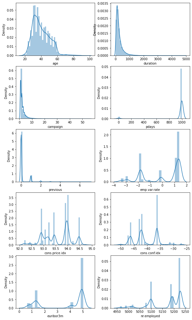
1# Distributions of numerical features
2plt.figure(figsize=(10, 18))
3for index, col in enumerate(numerical_features):
4    plt.subplot(5, 2, index + 1)
5    sns.distplot(dataset[col])
6plt.savefig(
7    f"{assets_path}/numerical_distributions.png", format="png", dpi=500
8)
1# Categorical features
2categorical_features = [
3    col
4    for col in dataset.columns
5    if pd.api.types.is_string_dtype(dataset[col])
6]
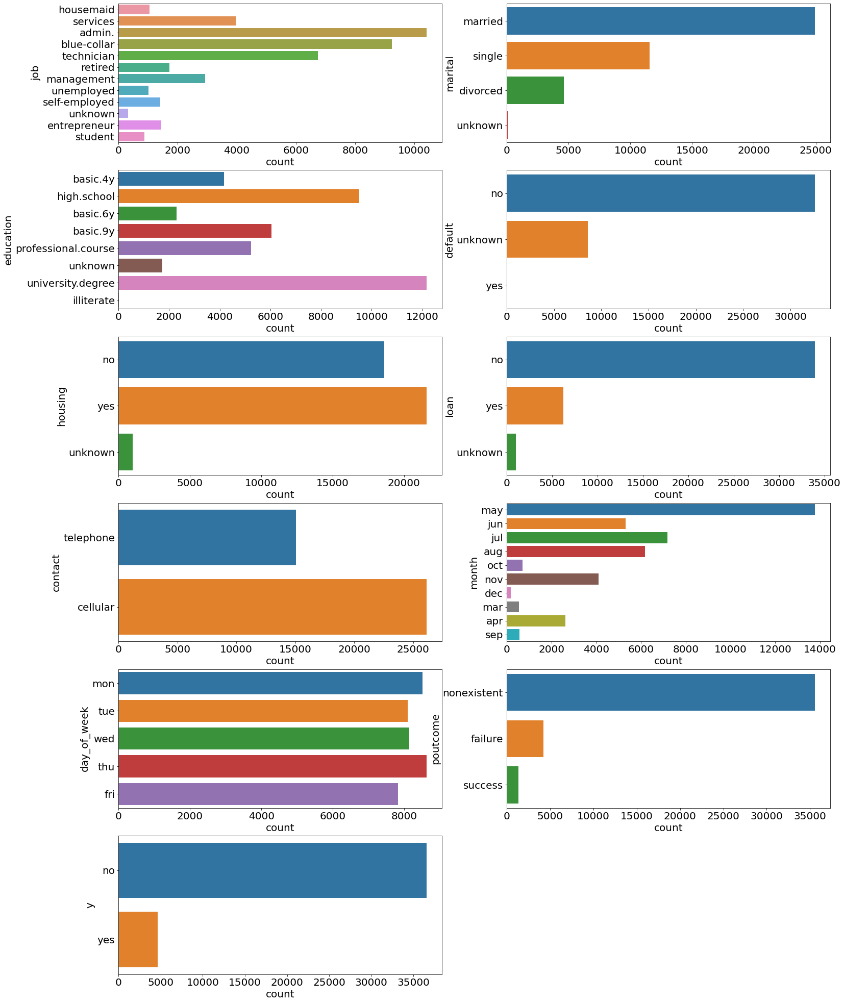
 1# Distributions of categorical features
 2plt.figure(figsize=(25, 35))
 3for index, col in enumerate(categorical_features):
 4    plt.subplot(6, 2, index + 1)
 5    ax = sns.countplot(y=col, data=dataset)
 6    ax.set_xlabel("count", fontsize=20)
 7    ax.set_ylabel(col, fontsize=20)
 8    ax.tick_params(labelsize=20)
 9
10plt.savefig(f"{assets_path}/categorical_counts.png", format="png", dpi=500)
1# Number of entries in y column
2print("Total number of entries:")
3print(dataset["y"].value_counts(ascending=True))
4print()
5print("Percentages:")
6print(dataset["y"].value_counts(normalize=True, ascending=True) * 100)
Total number of entries:
yes     4640
no     36548
Name: y, dtype: int64

Percentages:
yes    11.265417
no     88.734583
Name: y, dtype: float64
Linear regression on financial columns#
1# Feature matrix and target variable
2X = dataset[["emp.var.rate", "cons.price.idx", "euribor3m"]]
3X = sm.add_constant(X)  # add constant value for the intercept term
4y = dataset["cons.conf.idx"]
5
6# Defining and fitting model
7lineare_regression_model = sm.OLS(y, X)
8result = lineare_regression_model.fit()
9print(result.summary())
                            OLS Regression Results
==============================================================================
Dep. Variable:          cons.conf.idx   R-squared:                       0.177
Model:                            OLS   Adj. R-squared:                  0.177
Method:                 Least Squares   F-statistic:                     2960.
Date:                Mon, 11 Apr 2022   Prob (F-statistic):               0.00
Time:                        01:41:25   Log-Likelihood:            -1.1753e+05
No. Observations:               41188   AIC:                         2.351e+05
Df Residuals:                   41184   BIC:                         2.351e+05
Df Model:                           3
Covariance Type:            nonrobust
==================================================================================
                     coef    std err          t      P>|t|      [0.025      0.975]
----------------------------------------------------------------------------------
const            -82.4025      5.999    -13.736      0.000     -94.161     -70.644
emp.var.rate      -4.1814      0.072    -57.960      0.000      -4.323      -4.040
cons.price.idx     0.2828      0.063      4.478      0.000       0.159       0.407
euribor3m          4.3582      0.057     76.618      0.000       4.247       4.470
==============================================================================
Omnibus:                     3246.559   Durbin-Watson:                   0.001
Prob(Omnibus):                  0.000   Jarque-Bera (JB):             4034.493
Skew:                           0.761   Prob(JB):                         0.00
Kurtosis:                       2.811   Cond. No.                     2.72e+04
==============================================================================

Notes:
[1] Standard Errors assume that the covariance matrix of the errors is correctly specified.
[2] The condition number is large, 2.72e+04. This might indicate that there are
strong multicollinearity or other numerical problems.
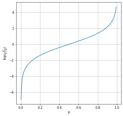
Logistic regression on campaign columns#
 1# Plotting logit function
 2x = np.arange(0.001, 1, 0.01)
 3logit = np.log(x / (1 - x))
 4
 5plt.figure(figsize=(6, 6))
 6plt.plot(x, logit)
 7plt.xlabel("p")
 8plt.ylabel(r"$\log(\frac{p}{1-p})$")
 9plt.grid()
10plt.savefig(f"{assets_path}/logit_function.png", format="png", dpi=300)
1# Feature matrix and target variable
2X = dataset[["age", "duration", "campaign", "previous"]]
3X = sm.add_constant(X)  # add constant value for the intercept term
4y = np.where(dataset["y"] == "yes", 1, 0)  # target has to be numeric
5
6# Defining and fitting model
7logistic_regression_model = sm.Logit(y, X)
8result = logistic_regression_model.fit()
9print(result.summary())
1# One hot encoding
2print(dataset["education"].unique())
3
4hot_encoded = pd.get_dummies(dataset["education"])
5hot_encoded["education"] = dataset["education"]
6hot_encoded.head(10)
Logistic regression on the full marketing campaign data#
1# Transforming all features into numerical ones using the
2# get_dummies() function
3X = dataset.drop("y", axis=1)
4X = pd.get_dummies(X)
5X = sm.add_constant(X)
6print(X.columns)
1# Extracting and transforming target variable
2y = np.where(dataset["y"] == "yes", 1, 0)
1# Defining and fitting model
2full_logistic_regression_model = sm.Logit(y, X)
3result = full_logistic_regression_model.fit(maxiter=500)
4print(result.summary())