

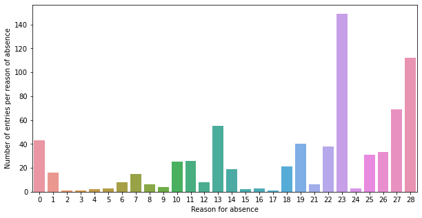
Initial analysis of reasons for absence#
First plots showing the overall distribution of the absence reasons in the data—that is, how many entries we have for a specific reason for absence in our dataset.
Importing libraries and packages#
 1# Mathematical operations and data manipulation
 2import pandas as pd
 3
 4# Plotting
 5import seaborn as sns
 6import matplotlib.pyplot as plt
 7
 8# Warnings
 9import warnings
10
11warnings.filterwarnings("ignore")
12
13%matplotlib inline
Set paths#
1# Path to datasets directory
2data_path = "./datasets"
3# Path to assets directory (for saving results to)
4assets_path = "./assets"
Loading dataset#
1# load data
2dataset = pd.read_csv(f"{data_path}/preprocessed_absenteism.csv")
3dataset.head()
| ID | Reason for absence | Month of absence | Day of the week | Seasons | Transportation expense | Distance from Residence to Work | Service time | Age | Work load Average/day | ... | Disciplinary failure | Education | Son | Social drinker | Social smoker | Pet | Weight | Height | Body mass index | Absenteeism time in hours | |
|---|---|---|---|---|---|---|---|---|---|---|---|---|---|---|---|---|---|---|---|---|---|
| 0 | 11 | 26 | July | Tuesday | Spring | 289 | 36 | 13 | 33 | 239.554 | ... | No | high_school | 2 | Yes | No | 1 | 90 | 172 | 30 | 4 |
| 1 | 36 | 0 | July | Tuesday | Spring | 118 | 13 | 18 | 50 | 239.554 | ... | Yes | high_school | 1 | Yes | No | 0 | 98 | 178 | 31 | 0 |
| 2 | 3 | 23 | July | Wednesday | Spring | 179 | 51 | 18 | 38 | 239.554 | ... | No | high_school | 0 | Yes | No | 0 | 89 | 170 | 31 | 2 |
| 3 | 7 | 7 | July | Thursday | Spring | 279 | 5 | 14 | 39 | 239.554 | ... | No | high_school | 2 | Yes | Yes | 0 | 68 | 168 | 24 | 4 |
| 4 | 11 | 23 | July | Thursday | Spring | 289 | 36 | 13 | 33 | 239.554 | ... | No | high_school | 2 | Yes | No | 1 | 90 | 172 | 30 | 2 |
5 rows × 21 columns
Exploring dataset#
1# Printing dimensionality of the data, columns, types and missing values
2print(f"Data dimension: {dataset.shape}")
3for col in dataset.columns:
4    print(
5        f"Column: {col:35} | "
6        f"type: {str(dataset[col].dtype):7} | "
7        f"missing values: {dataset[col].isna().sum():3d}"
8    )
Data dimension: (740, 21)
Column: ID                                  | type: int64   | missing values:   0
Column: Reason for absence                  | type: int64   | missing values:   0
Column: Month of absence                    | type: object  | missing values:   0
Column: Day of the week                     | type: object  | missing values:   0
Column: Seasons                             | type: object  | missing values:   0
Column: Transportation expense              | type: int64   | missing values:   0
Column: Distance from Residence to Work     | type: int64   | missing values:   0
Column: Service time                        | type: int64   | missing values:   0
Column: Age                                 | type: int64   | missing values:   0
Column: Work load Average/day               | type: float64 | missing values:   0
Column: Hit target                          | type: int64   | missing values:   0
Column: Disciplinary failure                | type: object  | missing values:   0
Column: Education                           | type: object  | missing values:   0
Column: Son                                 | type: int64   | missing values:   0
Column: Social drinker                      | type: object  | missing values:   0
Column: Social smoker                       | type: object  | missing values:   0
Column: Pet                                 | type: int64   | missing values:   0
Column: Weight                              | type: int64   | missing values:   0
Column: Height                              | type: int64   | missing values:   0
Column: Body mass index                     | type: int64   | missing values:   0
Column: Absenteeism time in hours           | type: int64   | missing values:   0
1# Computing statistics on numerical features
2dataset.describe().T
| count | mean | std | min | 25% | 50% | 75% | max | |
|---|---|---|---|---|---|---|---|---|
| ID | 740.0 | 18.017568 | 11.021247 | 1.000 | 9.000 | 18.000 | 28.000 | 36.000 |
| Reason for absence | 740.0 | 19.216216 | 8.433406 | 0.000 | 13.000 | 23.000 | 26.000 | 28.000 |
| Transportation expense | 740.0 | 221.329730 | 66.952223 | 118.000 | 179.000 | 225.000 | 260.000 | 388.000 |
| Distance from Residence to Work | 740.0 | 29.631081 | 14.836788 | 5.000 | 16.000 | 26.000 | 50.000 | 52.000 |
| Service time | 740.0 | 12.554054 | 4.384873 | 1.000 | 9.000 | 13.000 | 16.000 | 29.000 |
| Age | 740.0 | 36.450000 | 6.478772 | 27.000 | 31.000 | 37.000 | 40.000 | 58.000 |
| Work load Average/day | 740.0 | 271.490235 | 39.058116 | 205.917 | 244.387 | 264.249 | 294.217 | 378.884 |
| Hit target | 740.0 | 94.587838 | 3.779313 | 81.000 | 93.000 | 95.000 | 97.000 | 100.000 |
| Son | 740.0 | 1.018919 | 1.098489 | 0.000 | 0.000 | 1.000 | 2.000 | 4.000 |
| Pet | 740.0 | 0.745946 | 1.318258 | 0.000 | 0.000 | 0.000 | 1.000 | 8.000 |
| Weight | 740.0 | 79.035135 | 12.883211 | 56.000 | 69.000 | 83.000 | 89.000 | 108.000 |
| Height | 740.0 | 172.114865 | 6.034995 | 163.000 | 169.000 | 170.000 | 172.000 | 196.000 |
| Body mass index | 740.0 | 26.677027 | 4.285452 | 19.000 | 24.000 | 25.000 | 31.000 | 38.000 |
| Absenteeism time in hours | 740.0 | 6.924324 | 13.330998 | 0.000 | 2.000 | 3.000 | 8.000 | 120.000 |
Individual identification (ID)
Reason for absence (ICD). Absences attested by the International Code of Diseases (ICD) stratified into 21 categories (I to XXI) as follows:
I Certain infectious and parasitic diseases II Neoplasms III Diseases of the blood and blood-forming organs and certain disorders involving the immune mechanism IV Endocrine, nutritional and metabolic diseases V Mental and behavioural disorders VI Diseases of the nervous system VII Diseases of the eye and adnexa VIII Diseases of the ear and mastoid process IX Diseases of the circulatory system X Diseases of the respiratory system XI Diseases of the digestive system XII Diseases of the skin and subcutaneous tissue XIII Diseases of the musculoskeletal system and connective tissue XIV Diseases of the genitourinary system XV Pregnancy, childbirth and the puerperium XVI Certain conditions originating in the perinatal period XVII Congenital malformations, deformations and chromosomal abnormalities XVIII Symptoms, signs and abnormal clinical and laboratory findings, not elsewhere classified XIX Injury, poisoning and certain other consequences of external causes XX External causes of morbidity and mortality XXI Factors influencing health status and contact with health services.
And 7 categories without (CID) 2. patient follow-up (22), 3. medical consultation (23), 4. blood donation (24), 5. laboratory examination (25), 6. unjustified absence (26), 7. physiotherapy (27), 8. dental consultation (28).
Month of absence
Day of the week (Monday (2), Tuesday (3), Wednesday (4), Thursday (5), Friday (6))
Seasons (summer (1), autumn (2), winter (3), spring (4))
Transportation expense
Distance from Residence to Work (kilometers)
Service time
Age
Work load Average/day
Hit target
Disciplinary failure (yes=1; no=0)
Education (high school (1), graduate (2), postgraduate (3), master and doctor (4))
Son (number of children)
Social drinker (yes=1; no=0)
Social smoker (yes=1; no=0)
Pet (number of pet)
Weight
Height
Body mass index
Absenteeism time in hours (target)
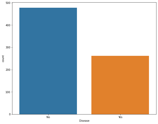
Reasons for absence#
 1# Function to chedatasetck if the provided integer value is contained
 2# in the ICD or not
 3def in_icd(val):
 4    r = range(1, 22)
 5    return "Yes" if val in r else "No"
 6
 7
 8# add Disease column
 9dataset["Disease"] = dataset["Reason for absence"].apply(in_icd)
10
11# plot value counts
12plt.figure(figsize=(10, 8))
13sns.countplot(data=dataset, x="Disease")
14plt.savefig(f"{assets_path}/disease_plot.png", format="png", dpi=300)
1# Plotting number of entries for each reason for absence
2plt.figure(figsize=(10, 5))
3ax = sns.countplot(data=dataset, x="Reason for absence")
4ax.set_ylabel("Number of entries per reason of absence")
5plt.savefig(
6    f"{assets_path}/absence_reasons_distribution.png", format="png", dpi=300
7)
 1# Plotting reasons for absence against being a social drinker/smoker
 2plt.figure(figsize=(8, 6))
 3sns.countplot(
 4    data=dataset,
 5    x="Reason for absence",
 6    hue="Social drinker",
 7    hue_order=["Yes", "No"],
 8)
 9plt.savefig(
10    f"{assets_path}/absence_reasons_drinkers.png", format="png", dpi=300
11)
12
13plt.figure(figsize=(8, 6))
14sns.countplot(
15    data=dataset,
16    x="Reason for absence",
17    hue="Social smoker",
18    hue_order=["Yes", "No"],
19)
20plt.savefig(
21    f"{assets_path}/absence_reasons_smokers.png", format="png", dpi=300
22)
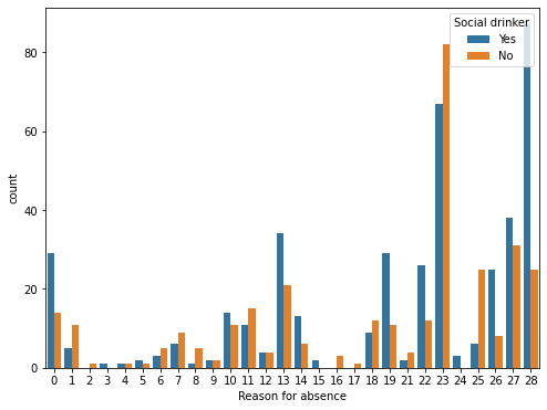
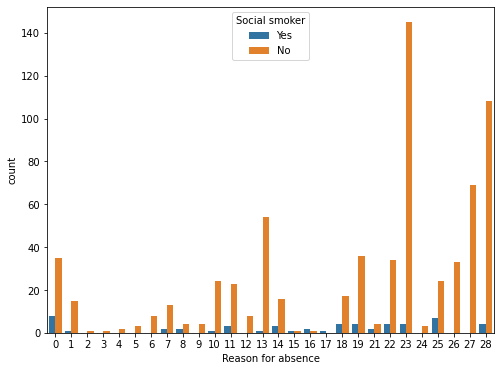
1# Calculating the actual count for social drinkers and smokers
2# from the preprocessed data
3print(dataset["Social drinker"].value_counts(normalize=True))
4print(dataset["Social smoker"].value_counts(normalize=True))
Yes    0.567568
No     0.432432
Name: Social drinker, dtype: float64
No     0.927027
Yes    0.072973
Name: Social smoker, dtype: float64