

Clustering#
Importing libraries and packages#
 1# Mathematical operations and data manipulation
 2import pandas as pd
 3
 4# Plotting
 5import matplotlib.pyplot as plt
 6
 7# Modelling
 8from sklearn.cluster import KMeans
 9
10# Warnings
11import warnings
12
13warnings.filterwarnings("ignore")
14
15%matplotlib inline
Set paths#
1# Path to datasets directory
2data_path = "./datasets"
3# Path to assets directory (for saving results to)
4assets_path = "./assets"
Loading dataset#
1# load data
2dataset = pd.read_csv(f"{data_path}/online_shoppers_intention.csv")
3dataset.head().T
| 0 | 1 | 2 | 3 | 4 | |
|---|---|---|---|---|---|
| Administrative | 0 | 0 | 0 | 0 | 0 |
| Administrative_Duration | 0.0 | 0.0 | 0.0 | 0.0 | 0.0 |
| Informational | 0 | 0 | 0 | 0 | 0 |
| Informational_Duration | 0.0 | 0.0 | 0.0 | 0.0 | 0.0 |
| ProductRelated | 1 | 2 | 1 | 2 | 10 |
| ProductRelated_Duration | 0.0 | 64.0 | 0.0 | 2.666667 | 627.5 |
| BounceRates | 0.2 | 0.0 | 0.2 | 0.05 | 0.02 |
| ExitRates | 0.2 | 0.1 | 0.2 | 0.14 | 0.05 |
| PageValues | 0.0 | 0.0 | 0.0 | 0.0 | 0.0 |
| SpecialDay | 0.0 | 0.0 | 0.0 | 0.0 | 0.0 |
| Month | Feb | Feb | Feb | Feb | Feb |
| OperatingSystems | 1 | 2 | 4 | 3 | 3 |
| Browser | 1 | 2 | 1 | 2 | 3 |
| Region | 1 | 1 | 9 | 2 | 1 |
| TrafficType | 1 | 2 | 3 | 4 | 4 |
| VisitorType | Returning_Visitor | Returning_Visitor | Returning_Visitor | Returning_Visitor | Returning_Visitor |
| Weekend | False | False | False | False | True |
| Revenue | False | False | False | False | False |
Exploring dataset#
1# Printing dimensionality of the data, columns, types and missing values
2print(f"Data dimension: {dataset.shape}")
3for col in dataset.columns:
4    print(
5        f"Column: {col:35} | "
6        f"type: {str(dataset[col].dtype):7} | "
7        f"missing values: {dataset[col].isna().sum():3d}"
8    )
Data dimension: (12330, 18)
Column: Administrative                      | type: int64   | missing values:   0
Column: Administrative_Duration             | type: float64 | missing values:   0
Column: Informational                       | type: int64   | missing values:   0
Column: Informational_Duration              | type: float64 | missing values:   0
Column: ProductRelated                      | type: int64   | missing values:   0
Column: ProductRelated_Duration             | type: float64 | missing values:   0
Column: BounceRates                         | type: float64 | missing values:   0
Column: ExitRates                           | type: float64 | missing values:   0
Column: PageValues                          | type: float64 | missing values:   0
Column: SpecialDay                          | type: float64 | missing values:   0
Column: Month                               | type: object  | missing values:   0
Column: OperatingSystems                    | type: int64   | missing values:   0
Column: Browser                             | type: int64   | missing values:   0
Column: Region                              | type: int64   | missing values:   0
Column: TrafficType                         | type: int64   | missing values:   0
Column: VisitorType                         | type: object  | missing values:   0
Column: Weekend                             | type: bool    | missing values:   0
Column: Revenue                             | type: bool    | missing values:   0
1# Computing statistics on numerical features
2dataset.describe().T
| count | mean | std | min | 25% | 50% | 75% | max | |
|---|---|---|---|---|---|---|---|---|
| Administrative | 12330.0 | 2.315166 | 3.321784 | 0.0 | 0.000000 | 1.000000 | 4.000000 | 27.000000 |
| Administrative_Duration | 12330.0 | 80.818611 | 176.779107 | 0.0 | 0.000000 | 7.500000 | 93.256250 | 3398.750000 |
| Informational | 12330.0 | 0.503569 | 1.270156 | 0.0 | 0.000000 | 0.000000 | 0.000000 | 24.000000 |
| Informational_Duration | 12330.0 | 34.472398 | 140.749294 | 0.0 | 0.000000 | 0.000000 | 0.000000 | 2549.375000 |
| ProductRelated | 12330.0 | 31.731468 | 44.475503 | 0.0 | 7.000000 | 18.000000 | 38.000000 | 705.000000 |
| ProductRelated_Duration | 12330.0 | 1194.746220 | 1913.669288 | 0.0 | 184.137500 | 598.936905 | 1464.157214 | 63973.522230 |
| BounceRates | 12330.0 | 0.022191 | 0.048488 | 0.0 | 0.000000 | 0.003112 | 0.016813 | 0.200000 |
| ExitRates | 12330.0 | 0.043073 | 0.048597 | 0.0 | 0.014286 | 0.025156 | 0.050000 | 0.200000 |
| PageValues | 12330.0 | 5.889258 | 18.568437 | 0.0 | 0.000000 | 0.000000 | 0.000000 | 361.763742 |
| SpecialDay | 12330.0 | 0.061427 | 0.198917 | 0.0 | 0.000000 | 0.000000 | 0.000000 | 1.000000 |
| OperatingSystems | 12330.0 | 2.124006 | 0.911325 | 1.0 | 2.000000 | 2.000000 | 3.000000 | 8.000000 |
| Browser | 12330.0 | 2.357097 | 1.717277 | 1.0 | 2.000000 | 2.000000 | 2.000000 | 13.000000 |
| Region | 12330.0 | 3.147364 | 2.401591 | 1.0 | 1.000000 | 3.000000 | 4.000000 | 9.000000 |
| TrafficType | 12330.0 | 4.069586 | 4.025169 | 1.0 | 2.000000 | 2.000000 | 4.000000 | 20.000000 |
Clustering#
K-means Clustering for Informational Duration versus Bounce Rate#
 1x = dataset.iloc[:, [3, 6]].values
 2
 3wcss = []
 4for i in range(1, 11):
 5    km = KMeans(
 6        n_clusters=i,
 7        init="k-means++",
 8        max_iter=300,
 9        n_init=10,
10        random_state=0,
11        algorithm="elkan",
12        tol=0.001,
13    )
14    km.fit(x)
15    labels = km.labels_
16    wcss.append(km.inertia_)
17
18plt.rcParams["figure.figsize"] = (15, 7)
19plt.plot(range(1, 11), wcss)
20plt.grid()
21plt.tight_layout()
22plt.title("The Elbow Method", fontsize=20)
23plt.xlabel("No. of Clusters")
24plt.ylabel("wcss")
25plt.show()
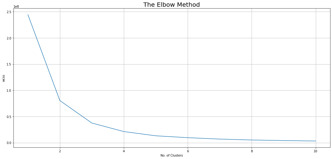
k=2 is the optimum value for clustering.
 1km = KMeans(
 2    n_clusters=2, init="k-means++", max_iter=300, n_init=10, random_state=0
 3)
 4y_means = km.fit_predict(x)
 5
 6plt.scatter(
 7    x[y_means == 0, 0],
 8    x[y_means == 0, 1],
 9    s=100,
10    c="pink",
11    label="Un-interested Customers",
12)
13plt.scatter(
14    x[y_means == 1, 0],
15    x[y_means == 1, 1],
16    s=100,
17    c="yellow",
18    label="Target Customers",
19)
20plt.scatter(
21    km.cluster_centers_[:, 0],
22    km.cluster_centers_[:, 1],
23    s=50,
24    c="blue",
25    label="centeroid",
26)
27
28plt.title("Informational Duration vs Bounce Rates", fontsize=20)
29plt.grid()
30plt.xlabel("Informational Duration")
31plt.ylabel("Bounce Rates")
32plt.legend()
33plt.show()
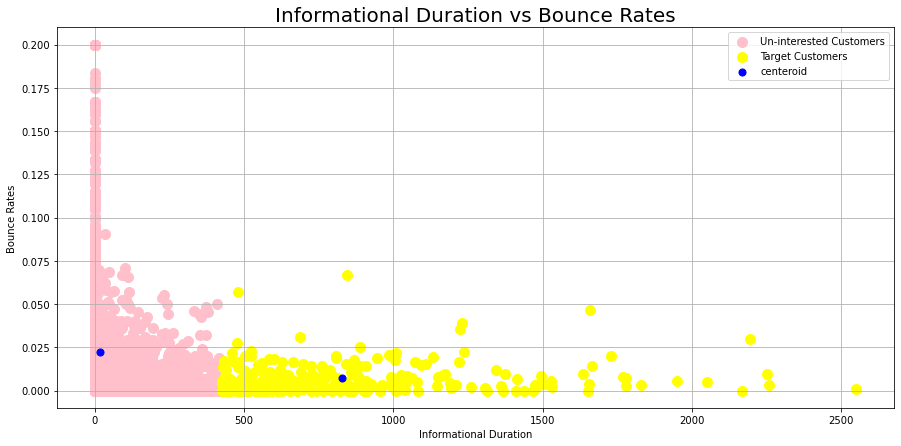
Target customers spend around 850-900 seconds on average on the Information page.
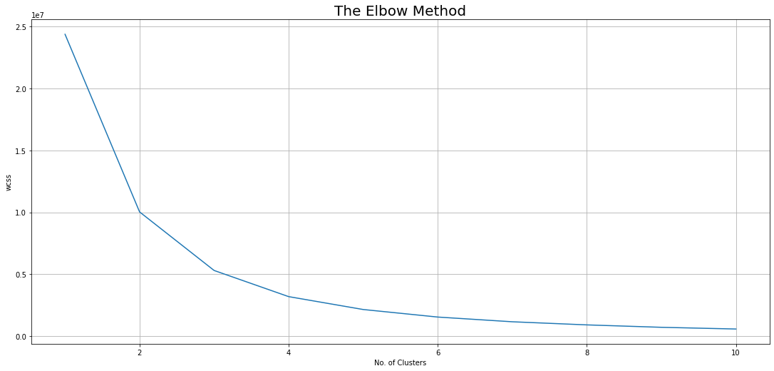
K-means Clustering for Informational Duration versus Exit Rate#
 1x = dataset.iloc[:, [4, 7]].values
 2
 3wcss = []
 4for i in range(1, 11):
 5    km = KMeans(
 6        n_clusters=i,
 7        init="k-means++",
 8        max_iter=300,
 9        n_init=10,
10        random_state=0,
11        algorithm="elkan",
12        tol=0.001,
13    )
14    km.fit(x)
15    labels = km.labels_
16    wcss.append(km.inertia_)
17
18plt.rcParams["figure.figsize"] = (15, 7)
19plt.plot(range(1, 11), wcss)
20plt.grid()
21plt.tight_layout()
22plt.title("The Elbow Method", fontsize=20)
23plt.xlabel("No. of Clusters")
24plt.ylabel("wcss")
25plt.show()
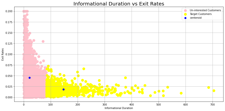
 1km = KMeans(
 2    n_clusters=2, init="k-means++", max_iter=300, n_init=10, random_state=0
 3)
 4y_means = km.fit_predict(x)
 5
 6plt.scatter(
 7    x[y_means == 0, 0],
 8    x[y_means == 0, 1],
 9    s=100,
10    c="pink",
11    label="Un-interested Customers",
12)
13plt.scatter(
14    x[y_means == 1, 0],
15    x[y_means == 1, 1],
16    s=100,
17    c="yellow",
18    label="Target Customers",
19)
20plt.scatter(
21    km.cluster_centers_[:, 0],
22    km.cluster_centers_[:, 1],
23    s=50,
24    c="blue",
25    label="centeroid",
26)
27
28plt.title("Informational Duration vs Exit Rates", fontsize=20)
29plt.grid()
30plt.xlabel("Informational Duration")
31plt.ylabel("Exit Rates")
32plt.legend()
33plt.show()
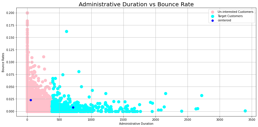
K-means Clustering for Administrative Duration versus Bounce Rate and Administrative Duration versus Exit Rate#
1# Administrative duration vs Bounce Rate
2x = dataset.iloc[:, [1, 6]].values
3x.shape
(12330, 2)
 1wcss = []
 2for i in range(1, 11):
 3    km = KMeans(
 4        n_clusters=i,
 5        init="k-means++",
 6        max_iter=300,
 7        n_init=10,
 8        random_state=0,
 9        algorithm="elkan",
10        tol=0.001,
11    )
12    km.fit(x)
13    labels = km.labels_
14    wcss.append(km.inertia_)
15
16plt.rcParams["figure.figsize"] = (15, 7)
17plt.plot(range(1, 11), wcss)
18plt.grid()
19plt.tight_layout()
20plt.title("The Elbow Method", fontsize=20)
21plt.xlabel("No. of Clusters")
22plt.ylabel("wcss")
23plt.show()

 1km = KMeans(
 2    n_clusters=2, init="k-means++", max_iter=300, n_init=10, random_state=0
 3)
 4y_means = km.fit_predict(x)
 5
 6plt.scatter(
 7    x[y_means == 0, 0],
 8    x[y_means == 0, 1],
 9    s=100,
10    c="pink",
11    label="Un-interested Customers",
12)
13plt.scatter(
14    x[y_means == 1, 0],
15    x[y_means == 1, 1],
16    s=100,
17    c="cyan",
18    label="Target Customers",
19)
20plt.scatter(
21    km.cluster_centers_[:, 0],
22    km.cluster_centers_[:, 1],
23    s=50,
24    c="blue",
25    label="centeroid",
26)
27
28plt.title("Administrative Duration vs Bounce Rate", fontsize=20)
29plt.grid()
30plt.xlabel("Administrative Duration")
31plt.ylabel("Bounce Rates")
32plt.legend()
33plt.show()
 1# Administrative duration vs Exit Rate
 2x = dataset.iloc[:, [1, 7]].values
 3
 4wcss = []
 5for i in range(1, 11):
 6    km = KMeans(
 7        n_clusters=i,
 8        init="k-means++",
 9        max_iter=300,
10        n_init=10,
11        random_state=0,
12        algorithm="elkan",
13        tol=0.001,
14    )
15    km.fit(x)
16    labels = km.labels_
17    wcss.append(km.inertia_)
18
19plt.rcParams["figure.figsize"] = (15, 7)
20plt.plot(range(1, 11), wcss)
21plt.grid()
22plt.tight_layout()
23plt.title("The Elbow Method", fontsize=20)
24plt.xlabel("No. of Clusters")
25plt.ylabel("wcss")
26plt.show()
 1km = KMeans(
 2    n_clusters=2, init="k-means++", max_iter=300, n_init=10, random_state=0
 3)
 4y_means = km.fit_predict(x)
 5
 6plt.scatter(
 7    x[y_means == 0, 0],
 8    x[y_means == 0, 1],
 9    s=100,
10    c="pink",
11    label="Un-interested Customers",
12)
13plt.scatter(
14    x[y_means == 1, 0],
15    x[y_means == 1, 1],
16    s=100,
17    c="yellow",
18    label="Target Customers",
19)
20plt.scatter(
21    km.cluster_centers_[:, 0],
22    km.cluster_centers_[:, 1],
23    s=50,
24    c="blue",
25    label="centeroid",
26)
27
28plt.title("Administrative Duration vs Exit Rates", fontsize=20)
29plt.grid()
30plt.xlabel("Administrative Duration")
31plt.ylabel("Exit Rates")
32plt.legend()
33plt.show()
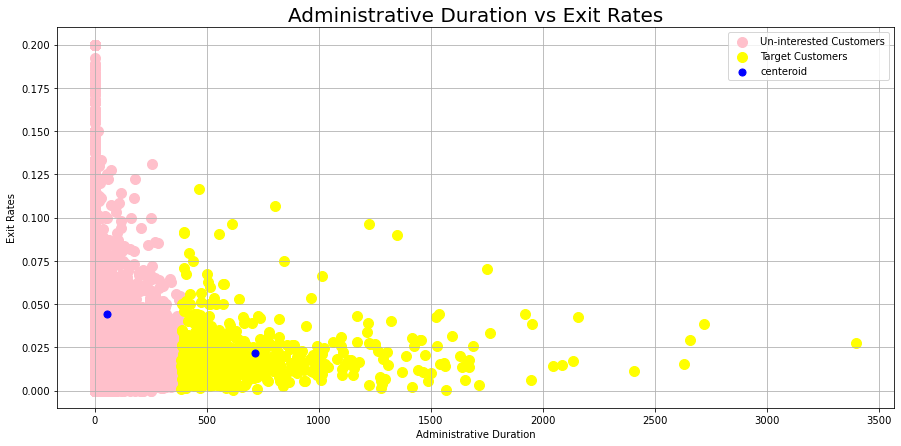
Uninterested customers spend less time in administrative pages compared with the target customers, who spend around 750 seconds on the administrative page before exiting.
The conversion rates of new visitors are high compared to those of returning customers.
While the number of returning customers to the website is high, the conversion rate is low compared to that of new customers.
Pages with a high page value have a lower bounce rate. We should be talking with our tech team to find ways to improve the page value of the web pages.