Hypothesis testing#
With hypothesis testing a general conclusion is made about a large group (a population) based on the analysis and measurements performed on a smaller group (a sample).
In general, a null hypothesis and a complementary alternative are defined, a test statistic whose value (a quantity calculated from the sample) is the basis for accepting or rejecting the null hypothesis is identified, and a significance level specified. Once a significance level is specified, the rejection points are computed, which are the values with which the test statistic is compared.
Importing libraries and packages#
 1# Warnings
 2import warnings
 3
 4# Mathematical operations and data manipulation
 5import pandas as pd
 6import random
 7
 8# Plotting
 9import seaborn as sns
10import matplotlib.pyplot as plt
11
12# Statistics
13from scipy.stats import ttest_1samp
14from scipy.stats import ttest_ind
15
16warnings.filterwarnings("ignore")
17%matplotlib inline
Set paths#
1# Path to datasets directory
2data_path = "./datasets"
3# Path to assets directory (for saving results to)
4assets_path = "./assets"
Loading dataset#
1# load hourly data
2dataset = pd.read_csv(f"{data_path}/preprocessed_hour.csv")
3dataset.head()
| instant | dteday | season | yr | mnth | hr | holiday | weekday | workingday | weathersit | temp | atemp | hum | windspeed | casual | registered | cnt | |
|---|---|---|---|---|---|---|---|---|---|---|---|---|---|---|---|---|---|
| 0 | 1 | 2011-01-01 | winter | 2011 | 1 | 0 | 0 | Saturday | 0 | clear | 0.24 | 0.2879 | 81.0 | 0.0 | 3 | 13 | 16 |
| 1 | 2 | 2011-01-01 | winter | 2011 | 1 | 1 | 0 | Saturday | 0 | clear | 0.22 | 0.2727 | 80.0 | 0.0 | 8 | 32 | 40 |
| 2 | 3 | 2011-01-01 | winter | 2011 | 1 | 2 | 0 | Saturday | 0 | clear | 0.22 | 0.2727 | 80.0 | 0.0 | 5 | 27 | 32 |
| 3 | 4 | 2011-01-01 | winter | 2011 | 1 | 3 | 0 | Saturday | 0 | clear | 0.24 | 0.2879 | 75.0 | 0.0 | 3 | 10 | 13 |
| 4 | 5 | 2011-01-01 | winter | 2011 | 1 | 4 | 0 | Saturday | 0 | clear | 0.24 | 0.2879 | 75.0 | 0.0 | 0 | 1 | 1 |
1# print some generic statistics about the data
2print(f"Shape of data: {dataset.shape}")
3print(f"Number of missing values in the data: {dataset.isnull().sum().sum()}")
4
5# get statistics on the numerical columns
6dataset.describe().T
Shape of data: (17379, 17)
Number of missing values in the data: 0
| count | mean | std | min | 25% | 50% | 75% | max | |
|---|---|---|---|---|---|---|---|---|
| instant | 17379.0 | 8690.000000 | 5017.029500 | 1.00 | 4345.5000 | 8690.0000 | 13034.5000 | 17379.0000 |
| yr | 17379.0 | 2011.502561 | 0.500008 | 2011.00 | 2011.0000 | 2012.0000 | 2012.0000 | 2012.0000 |
| mnth | 17379.0 | 6.537775 | 3.438776 | 1.00 | 4.0000 | 7.0000 | 10.0000 | 12.0000 |
| hr | 17379.0 | 11.546752 | 6.914405 | 0.00 | 6.0000 | 12.0000 | 18.0000 | 23.0000 |
| holiday | 17379.0 | 0.028770 | 0.167165 | 0.00 | 0.0000 | 0.0000 | 0.0000 | 1.0000 |
| workingday | 17379.0 | 0.682721 | 0.465431 | 0.00 | 0.0000 | 1.0000 | 1.0000 | 1.0000 |
| temp | 17379.0 | 0.496987 | 0.192556 | 0.02 | 0.3400 | 0.5000 | 0.6600 | 1.0000 |
| atemp | 17379.0 | 0.475775 | 0.171850 | 0.00 | 0.3333 | 0.4848 | 0.6212 | 1.0000 |
| hum | 17379.0 | 62.722884 | 19.292983 | 0.00 | 48.0000 | 63.0000 | 78.0000 | 100.0000 |
| windspeed | 17379.0 | 12.736540 | 8.196795 | 0.00 | 7.0015 | 12.9980 | 16.9979 | 56.9969 |
| casual | 17379.0 | 35.676218 | 49.305030 | 0.00 | 4.0000 | 17.0000 | 48.0000 | 367.0000 |
| registered | 17379.0 | 153.786869 | 151.357286 | 0.00 | 34.0000 | 115.0000 | 220.0000 | 886.0000 |
| cnt | 17379.0 | 189.463088 | 181.387599 | 1.00 | 40.0000 | 142.0000 | 281.0000 | 977.0000 |
Estimating average registered rides#
 1# Computing population mean of registered rides
 2population_mean = dataset.registered.mean()
 3
 4# Sample of the data (summer 2011)
 5sample = dataset[
 6    (dataset.season == "summer") & (dataset.yr == 2011)
 7].registered
 8
 9# t-test and computing p-value
10test_result = ttest_1samp(sample, population_mean)
11print(
12    f"Test statistic: {test_result[0]:.03f}, "
13    f"p-value: {test_result[1]:.03f}"
14)
15
16# Sample as 5% of the full data
17random.seed(111)
18sample_unbiased = dataset.registered.sample(frac=0.05)
19test_result_unbiased = ttest_1samp(sample_unbiased, population_mean)
20print(
21    f"Unbiased test statistic: {test_result_unbiased[0]:.03f}, "
22    f"p-value: {test_result_unbiased[1]:.03f}"
23)
Test statistic: -3.492, p-value: 0.000
Unbiased test statistic: -0.874, p-value: 0.382
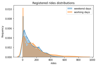
Hypothesis testing on registered rides#
 1# Defining mask, indicating if the day is weekend or work day
 2weekend_days = ["Saturday", "Sunday"]
 3weekend_mask = dataset.weekday.isin(weekend_days)
 4workingdays_mask = ~dataset.weekday.isin(weekend_days)
 5
 6# Selecting registered rides for the weekend and working days
 7weekend_data = dataset.registered[weekend_mask]
 8workingdays_data = dataset.registered[workingdays_mask]
 9
10# t-test
11test_res = ttest_ind(weekend_data, workingdays_data)
12print(f"Statistic value: {test_res[0]:.03f}, p-value: {test_res[1]:.03f}")
13
14# Plotting distributions of registered rides for working vs weekend days
15sns.distplot(weekend_data, label="weekend days")
16sns.distplot(workingdays_data, label="working days")
17plt.legend()
18plt.xlabel("rides")
19plt.ylabel("frequency")
20plt.title("Registered rides distributions")
21plt.savefig(f"{assets_path}/hypothesis_testing_a.png", format="png")
Statistic value: -16.004, p-value: 0.000
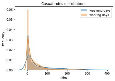
 1# Selecting casual rides for the weekend and working days
 2weekend_data = dataset.casual[weekend_mask]
 3workingdays_data = dataset.casual[workingdays_mask]
 4
 5# t-test
 6test_res = ttest_ind(weekend_data, workingdays_data)
 7print(f"Statistic value: {test_res[0]:.03f}, p-value: {test_res[1]:.03f}")
 8
 9# Plotting distributions of casual rides for working vs weekend days
10sns.distplot(weekend_data, label="weekend days")
11sns.distplot(workingdays_data, label="working days")
12plt.legend()
13plt.xlabel("rides")
14plt.ylabel("frequency")
15plt.title("Casual rides distributions")
16plt.savefig(f"{assets_path}/hypothesis_testing_b.png", format="png")
Statistic value: 41.077, p-value: 0.000