Exploratory data analysis

Importing libraries and packages

# Mathematical operations and data manipulation
import numpy as np
import pandas as pd

# Plotting
import seaborn as sns
import matplotlib.pyplot as plt
import plotly.graph_objs as go

# Warnings
import warnings

warnings.filterwarnings("ignore")

%matplotlib inline

Set paths

# Path to datasets directory
data_path = "./datasets"
# Path to assets directory (for saving results to)
assets_path = "./assets"

Loading dataset

# load data
dataset = pd.read_csv(f"{data_path}/engineered_energydata.csv")
dataset.head().T

	0	1	2	3	4
date_time	2016-01-11 17:00:00	2016-01-11 17:10:00	2016-01-11 17:20:00	2016-01-11 17:30:00	2016-01-11 17:40:00
month	1	1	1	1	1
day	1	1	1	1	1
a_energy	60	60	50	50	60
kitchen_temp	19.89	19.89	19.89	19.89	19.89
kitchen_hum	47.596667	46.693333	46.3	46.066667	46.333333
liv_temp	19.2	19.2	19.2	19.2	19.2
liv_hum	44.79	44.7225	44.626667	44.59	44.53
laun_temp	19.79	19.79	19.79	19.79	19.79
laun_hum	44.73	44.79	44.933333	45.0	45.0
off_temp	19.0	19.0	18.926667	18.89	18.89
off_hum	45.566667	45.9925	45.89	45.723333	45.53
bath_temp	17.166667	17.166667	17.166667	17.166667	17.2
bath_hum	55.2	55.2	55.09	55.09	55.09
out_b_temp	7.026667	6.833333	6.56	6.433333	6.366667
out_b_hum	84.256667	84.063333	83.156667	83.423333	84.893333
iron_temp	17.2	17.2	17.2	17.133333	17.2
iron_hum	41.626667	41.56	41.433333	41.29	41.23
teen_temp	18.2	18.2	18.2	18.1	18.1
teen_hum	48.9	48.863333	48.73	48.59	48.59
par_temp	17.033333	17.066667	17.0	17.0	17.0
par_hum	45.53	45.56	45.5	45.4	45.4
out_temp	6.6	6.483333	6.366667	6.25	6.133333
out_press	733.5	733.6	733.7	733.8	733.9
out_hum	92.0	92.0	92.0	92.0	92.0
wind	7.0	6.666667	6.333333	6.0	5.666667
visibility	63.0	59.166667	55.333333	51.5	47.666667
dew_point	5.3	5.2	5.1	5.0	4.9
rv1	13.275433	18.606195	28.642668	45.410389	10.084097
rv2	13.275433	18.606195	28.642668	45.410389	10.084097

Data analysis

Visualizing the Dataset

app_date = go.Scatter(x=dataset.date_time, mode="lines", y=dataset.a_energy)

layout = go.Layout(
    title="Appliance Energy Consumed by Date",
    xaxis=dict(title="Date"),
    yaxis=dict(title="Wh"),
)
fig = go.Figure(data=[app_date], layout=layout)
fig.show()

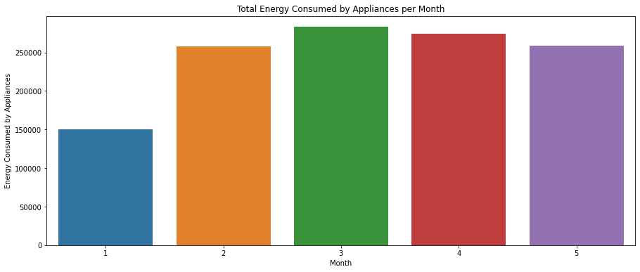
app_mon = dataset.groupby(by=["month"], as_index=False)["a_energy"].sum()
app_mon.sort_values(by="a_energy", ascending=False).head()

	month	a_energy
2	3	283190
3	4	274030
4	5	259120
1	2	258270
0	1	150060

plt.subplots(figsize=(15, 6))
am = sns.barplot(app_mon.month, app_mon.a_energy)
plt.xlabel("Month")
plt.ylabel("Energy Consumed by Appliances")
plt.title("Total Energy Consumed by Appliances per Month")
plt.show()

Observing the Trend between a_energy and day

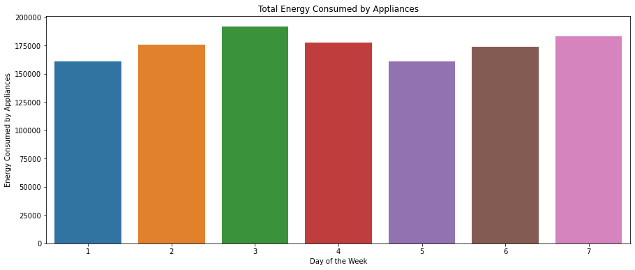
app_day = dataset.groupby(by=["day"], as_index=False)["a_energy"].sum()
app_day.sort_values(by="a_energy", ascending=False)

	day	a_energy
2	3	191700
6	7	183210
3	4	177830
1	2	175930
5	6	173640
0	1	161190
4	5	161170

plt.subplots(figsize=(15, 6))
ad = sns.barplot(app_day.day, app_day.a_energy)
plt.xlabel("Day of the Week")
plt.ylabel("Energy Consumed by Appliances")
plt.title("Total Energy Consumed by Appliances")
plt.show()

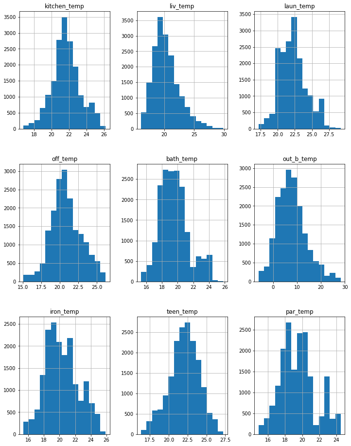
Distributions of the Temperature Columns

col_temp = [
    "kitchen_temp",
    "liv_temp",
    "laun_temp",
    "off_temp",
    "bath_temp",
    "out_b_temp",
    "iron_temp",
    "teen_temp",
    "par_temp",
]
temp = dataset[col_temp]
temp.head()

	kitchen_temp	liv_temp	laun_temp	off_temp	bath_temp	out_b_temp	iron_temp	teen_temp	par_temp
0	19.89	19.2	19.79	19.000000	17.166667	7.026667	17.200000	18.2	17.033333
1	19.89	19.2	19.79	19.000000	17.166667	6.833333	17.200000	18.2	17.066667
2	19.89	19.2	19.79	18.926667	17.166667	6.560000	17.200000	18.2	17.000000
3	19.89	19.2	19.79	18.890000	17.166667	6.433333	17.133333	18.1	17.000000
4	19.89	19.2	19.79	18.890000	17.200000	6.366667	17.200000	18.1	17.000000

temp.hist(bins=15, figsize=(12, 16))

array([[<AxesSubplot:title={'center':'kitchen_temp'}>,
        <AxesSubplot:title={'center':'liv_temp'}>,
        <AxesSubplot:title={'center':'laun_temp'}>],
       [<AxesSubplot:title={'center':'off_temp'}>,
        <AxesSubplot:title={'center':'bath_temp'}>,
        <AxesSubplot:title={'center':'out_b_temp'}>],
       [<AxesSubplot:title={'center':'iron_temp'}>,
        <AxesSubplot:title={'center':'teen_temp'}>,
        <AxesSubplot:title={'center':'par_temp'}>]], dtype=object)

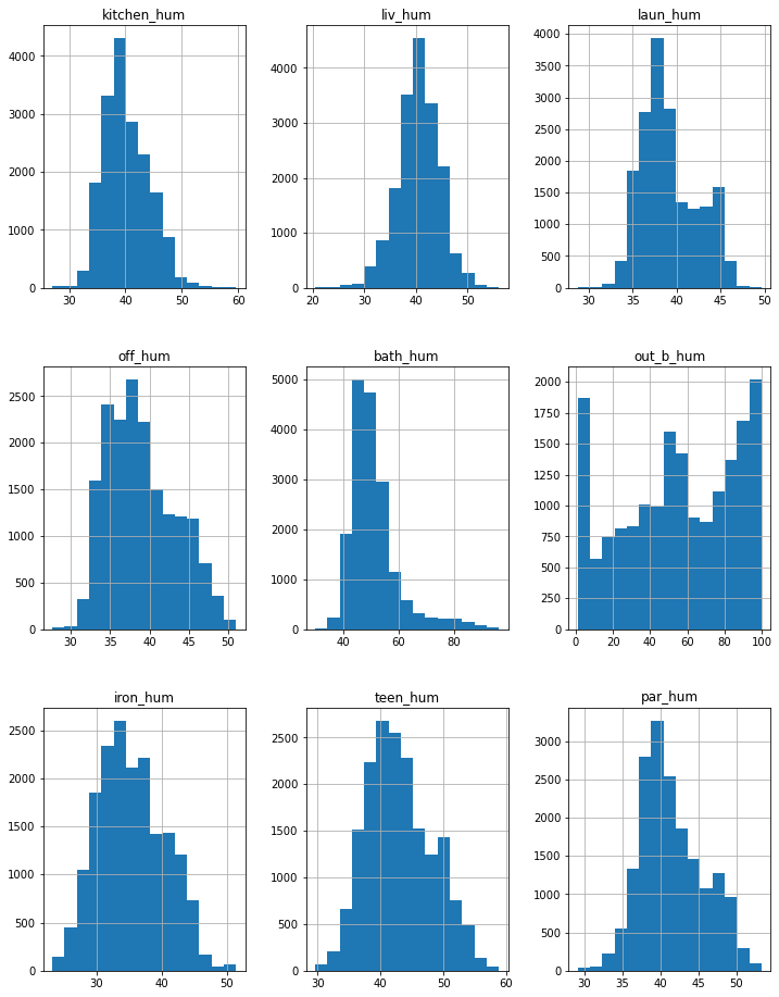
Distributions of the Humidity Columns

col_hum = [
    "kitchen_hum",
    "liv_hum",
    "laun_hum",
    "off_hum",
    "bath_hum",
    "out_b_hum",
    "iron_hum",
    "teen_hum",
    "par_hum",
]
hum = dataset[col_hum]
hum.head()

	kitchen_hum	liv_hum	laun_hum	off_hum	bath_hum	out_b_hum	iron_hum	teen_hum	par_hum
0	47.596667	44.790000	44.730000	45.566667	55.20	84.256667	41.626667	48.900000	45.53
1	46.693333	44.722500	44.790000	45.992500	55.20	84.063333	41.560000	48.863333	45.56
2	46.300000	44.626667	44.933333	45.890000	55.09	83.156667	41.433333	48.730000	45.50
3	46.066667	44.590000	45.000000	45.723333	55.09	83.423333	41.290000	48.590000	45.40
4	46.333333	44.530000	45.000000	45.530000	55.09	84.893333	41.230000	48.590000	45.40

hum.hist(bins=15, figsize=(12, 16))

array([[<AxesSubplot:title={'center':'kitchen_hum'}>,
        <AxesSubplot:title={'center':'liv_hum'}>,
        <AxesSubplot:title={'center':'laun_hum'}>],
       [<AxesSubplot:title={'center':'off_hum'}>,
        <AxesSubplot:title={'center':'bath_hum'}>,
        <AxesSubplot:title={'center':'out_b_hum'}>],
       [<AxesSubplot:title={'center':'iron_hum'}>,
        <AxesSubplot:title={'center':'teen_hum'}>,
        <AxesSubplot:title={'center':'par_hum'}>]], dtype=object)

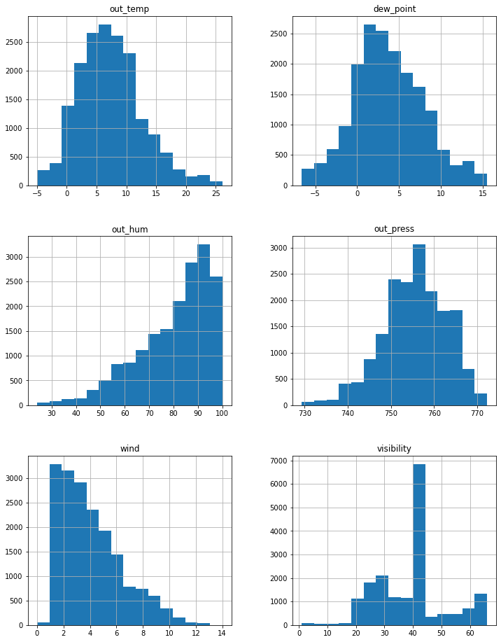
col_weather = [
    "out_temp",
    "dew_point",
    "out_hum",
    "out_press",
    "wind",
    "visibility",
]
weath = dataset[col_weather]
weath.head()

	out_temp	dew_point	out_hum	out_press	wind	visibility
0	6.600000	5.3	92.0	733.5	7.000000	63.000000
1	6.483333	5.2	92.0	733.6	6.666667	59.166667
2	6.366667	5.1	92.0	733.7	6.333333	55.333333
3	6.250000	5.0	92.0	733.8	6.000000	51.500000
4	6.133333	4.9	92.0	733.9	5.666667	47.666667

weath.hist(bins=15, figsize=(12, 16))

array([[<AxesSubplot:title={'center':'out_temp'}>,
        <AxesSubplot:title={'center':'dew_point'}>],
       [<AxesSubplot:title={'center':'out_hum'}>,
        <AxesSubplot:title={'center':'out_press'}>],
       [<AxesSubplot:title={'center':'wind'}>,
        <AxesSubplot:title={'center':'visibility'}>]], dtype=object)

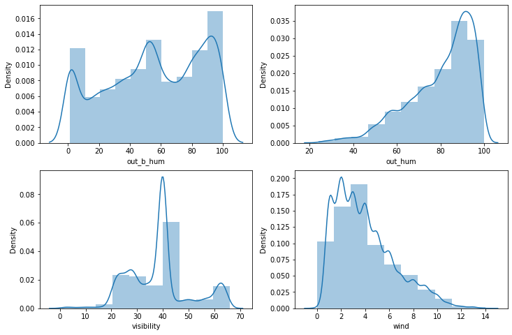
Plotting out_b, out_hum, visibility, and wind

f, ax = plt.subplots(2, 2, figsize=(12, 8))
obh = sns.distplot(hum["out_b_hum"], bins=10, ax=ax[0][0])
oh = sns.distplot(weath["out_hum"], bins=10, ax=ax[0][1])
vis = sns.distplot(weath["visibility"], bins=10, ax=ax[1][0])
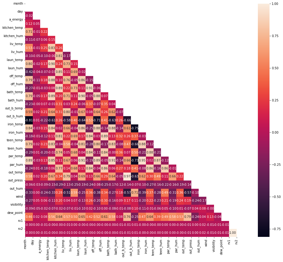
wind = sns.distplot(weath["wind"], bins=10, ax=ax[1][1])

corr = dataset.corr()
mask = np.zeros_like(corr, dtype=np.bool)
mask[np.triu_indices_from(mask)] = True
f, ax = plt.subplots(figsize=(16, 14))
sns.heatmap(corr, annot=True, fmt=".2f", mask=mask)
plt.xticks(range(len(corr.columns)), corr.columns)
plt.yticks(range(len(corr.columns)), corr.columns)
plt.show()