

Impact of numerical features on the outcome#
Loading the data and performing some initial exploration on it to acquire some basic knowledge about the data, how the various features are distributed.
Importing libraries and packages#
 1# Mathematical operations and data manipulation
 2import numpy as np
 3import pandas as pd
 4
 5# Statistics
 6from scipy.stats import ttest_ind
 7from scipy.stats import ks_2samp
 8
 9# Plotting
10import seaborn as sns
11import matplotlib.pyplot as plt
12
13# Warnings
14import warnings
15
16warnings.filterwarnings("ignore")
17
18%matplotlib inline
Set paths#
1# Path to datasets directory
2data_path = "./datasets"
3# Path to assets directory (for saving results to)
4assets_path = "./assets"
Loading dataset#
1# load data
2dataset = pd.read_csv(f"{data_path}/bank-additional-full.csv", sep=";")
3dataset.head().T
| 0 | 1 | 2 | 3 | 4 | |
|---|---|---|---|---|---|
| age | 56 | 57 | 37 | 40 | 56 |
| job | housemaid | services | services | admin. | services |
| marital | married | married | married | married | married |
| education | basic.4y | high.school | high.school | basic.6y | high.school |
| default | no | unknown | no | no | no |
| housing | no | no | yes | no | no |
| loan | no | no | no | no | yes |
| contact | telephone | telephone | telephone | telephone | telephone |
| month | may | may | may | may | may |
| day_of_week | mon | mon | mon | mon | mon |
| duration | 261 | 149 | 226 | 151 | 307 |
| campaign | 1 | 1 | 1 | 1 | 1 |
| pdays | 999 | 999 | 999 | 999 | 999 |
| previous | 0 | 0 | 0 | 0 | 0 |
| poutcome | nonexistent | nonexistent | nonexistent | nonexistent | nonexistent |
| emp.var.rate | 1.1 | 1.1 | 1.1 | 1.1 | 1.1 |
| cons.price.idx | 93.994 | 93.994 | 93.994 | 93.994 | 93.994 |
| cons.conf.idx | -36.4 | -36.4 | -36.4 | -36.4 | -36.4 |
| euribor3m | 4.857 | 4.857 | 4.857 | 4.857 | 4.857 |
| nr.employed | 5191.0 | 5191.0 | 5191.0 | 5191.0 | 5191.0 |
| y | no | no | no | no | no |
Exploring dataset#
1# Printing dimensionality of the data, columns, types and missing values
2print(f"Data dimension: {dataset.shape}")
3for col in dataset.columns:
4    print(
5        f"Column: {col:35} | "
6        f"type: {str(dataset[col].dtype):7} | "
7        f"missing values: {dataset[col].isna().sum():3d}"
8    )
Data dimension: (41188, 21)
Column: age                                 | type: int64   | missing values:   0
Column: job                                 | type: object  | missing values:   0
Column: marital                             | type: object  | missing values:   0
Column: education                           | type: object  | missing values:   0
Column: default                             | type: object  | missing values:   0
Column: housing                             | type: object  | missing values:   0
Column: loan                                | type: object  | missing values:   0
Column: contact                             | type: object  | missing values:   0
Column: month                               | type: object  | missing values:   0
Column: day_of_week                         | type: object  | missing values:   0
Column: duration                            | type: int64   | missing values:   0
Column: campaign                            | type: int64   | missing values:   0
Column: pdays                               | type: int64   | missing values:   0
Column: previous                            | type: int64   | missing values:   0
Column: poutcome                            | type: object  | missing values:   0
Column: emp.var.rate                        | type: float64 | missing values:   0
Column: cons.price.idx                      | type: float64 | missing values:   0
Column: cons.conf.idx                       | type: float64 | missing values:   0
Column: euribor3m                           | type: float64 | missing values:   0
Column: nr.employed                         | type: float64 | missing values:   0
Column: y                                   | type: object  | missing values:   0
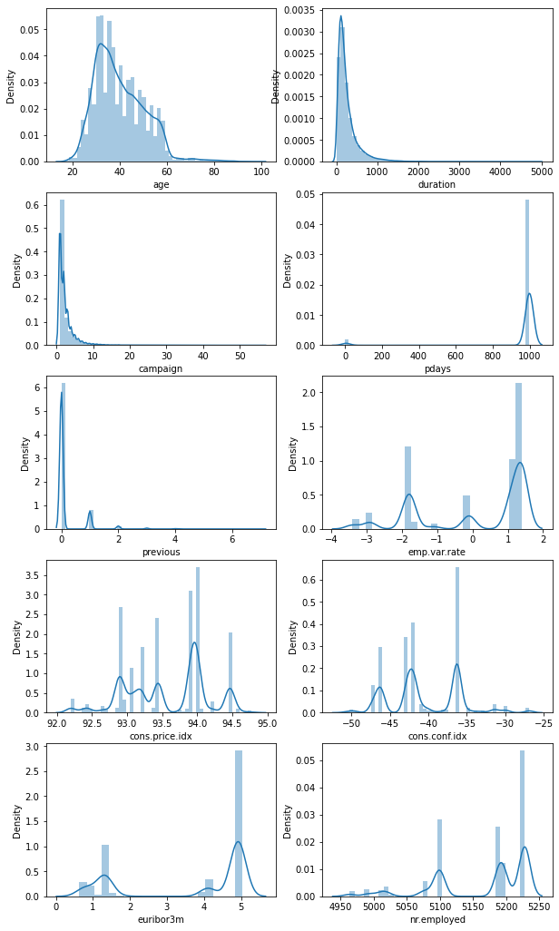
1# Numerical features
2numerical_features = [
3    col
4    for col in dataset.columns
5    if np.issubdtype(dataset[col].dtype, np.number)
6]
7print(numerical_features)
['age', 'duration', 'campaign', 'pdays', 'previous', 'emp.var.rate', 'cons.price.idx', 'cons.conf.idx', 'euribor3m', 'nr.employed']
1# Computing statistics on numerical features
2dataset[numerical_features].describe().T
| count | mean | std | min | 25% | 50% | 75% | max | |
|---|---|---|---|---|---|---|---|---|
| age | 41188.0 | 40.024060 | 10.421250 | 17.000 | 32.000 | 38.000 | 47.000 | 98.000 |
| duration | 41188.0 | 258.285010 | 259.279249 | 0.000 | 102.000 | 180.000 | 319.000 | 4918.000 |
| campaign | 41188.0 | 2.567593 | 2.770014 | 1.000 | 1.000 | 2.000 | 3.000 | 56.000 |
| pdays | 41188.0 | 962.475454 | 186.910907 | 0.000 | 999.000 | 999.000 | 999.000 | 999.000 |
| previous | 41188.0 | 0.172963 | 0.494901 | 0.000 | 0.000 | 0.000 | 0.000 | 7.000 |
| emp.var.rate | 41188.0 | 0.081886 | 1.570960 | -3.400 | -1.800 | 1.100 | 1.400 | 1.400 |
| cons.price.idx | 41188.0 | 93.575664 | 0.578840 | 92.201 | 93.075 | 93.749 | 93.994 | 94.767 |
| cons.conf.idx | 41188.0 | -40.502600 | 4.628198 | -50.800 | -42.700 | -41.800 | -36.400 | -26.900 |
| euribor3m | 41188.0 | 3.621291 | 1.734447 | 0.634 | 1.344 | 4.857 | 4.961 | 5.045 |
| nr.employed | 41188.0 | 5167.035911 | 72.251528 | 4963.600 | 5099.100 | 5191.000 | 5228.100 | 5228.100 |
1# Distributions of numerical features
2plt.figure(figsize=(10, 18))
3for index, col in enumerate(numerical_features):
4    plt.subplot(5, 2, index + 1)
5    sns.distplot(dataset[col])
6plt.savefig(
7    f"{assets_path}/numerical_distributions.png", format="png", dpi=500
8)
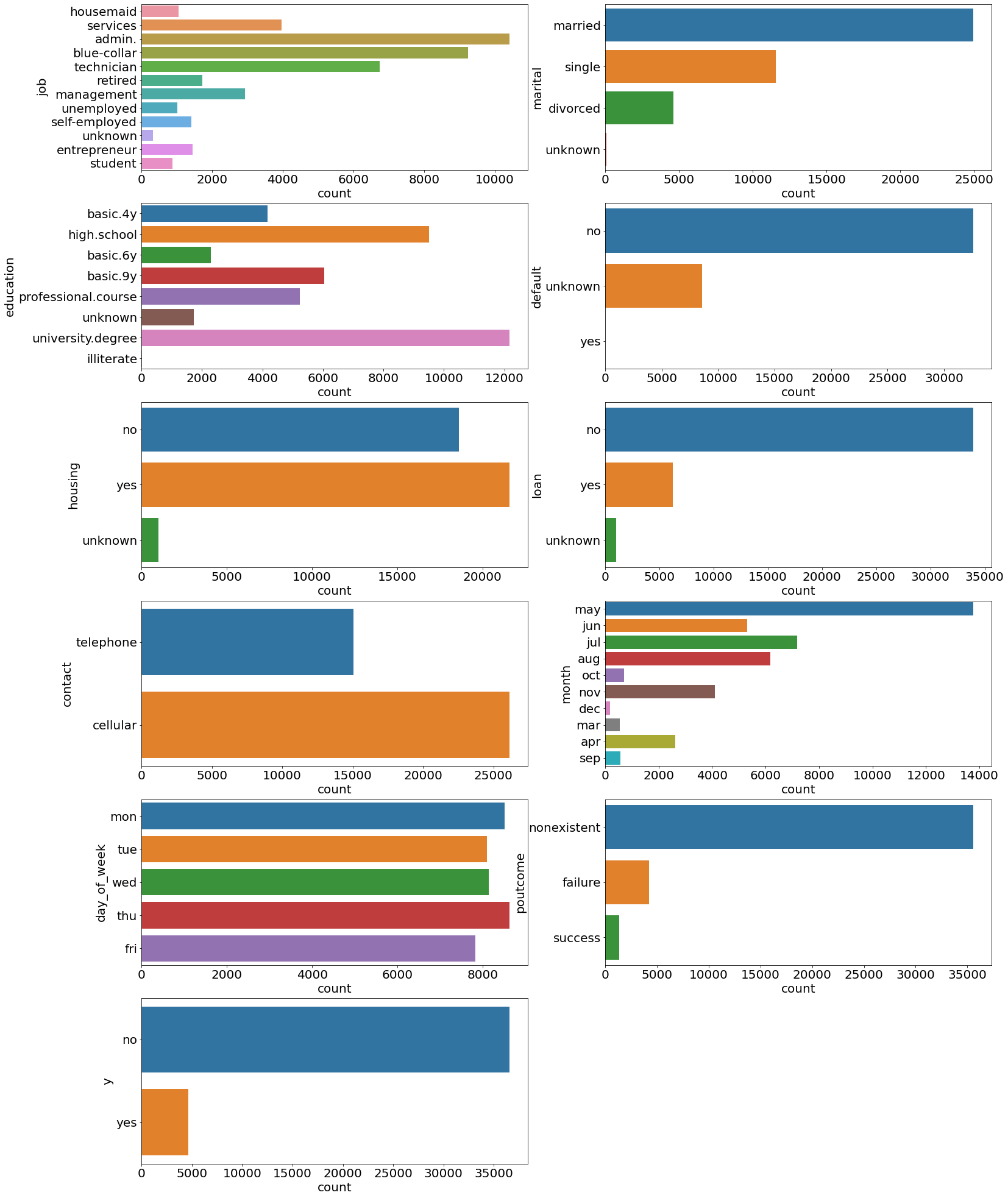
1# Categorical features
2categorical_features = [
3    col
4    for col in dataset.columns
5    if pd.api.types.is_string_dtype(dataset[col])
6]
 1# Distributions of categorical features
 2plt.figure(figsize=(25, 35))
 3for index, col in enumerate(categorical_features):
 4    plt.subplot(6, 2, index + 1)
 5    ax = sns.countplot(y=col, data=dataset)
 6    ax.set_xlabel("count", fontsize=20)
 7    ax.set_ylabel(col, fontsize=20)
 8    ax.tick_params(labelsize=20)
 9
10plt.savefig(f"{assets_path}/categorical_counts.png", format="png", dpi=500)
Analysis#
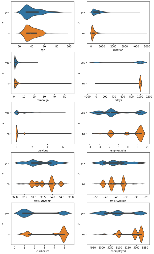
Is there a statistically significant difference in numerical features for successful and non-successful marketing campaigns?
1# Violin plots of numerical features against the outcome (y)
2# of the marketing campaign
3plt.figure(figsize=(10, 18))
4for index, col in enumerate(numerical_features):
5    plt.subplot(5, 2, index + 1)
6    sns.violinplot(x=col, y="y", data=dataset, order=["yes", "no"])
7plt.savefig(
8    f"{assets_path}/violin_plots_numerical_features.png", format="png", dpi=500
9)
 1# Function for computing mean of column for yes and no cases,
 2# and the test statistics and pvalue for equality of means test
 3def test_means(data, column):
 4    yes_mask = data["y"] == "yes"
 5    values_yes = data[column][yes_mask]
 6    values_no = data[column][~yes_mask]
 7    mean_yes = values_yes.mean()
 8    mean_no = values_no.mean()
 9
10    ttest_res = ttest_ind(values_yes, values_no)
11
12    return [
13        column,
14        mean_yes,
15        mean_no,
16        round(ttest_res[0], 4),
17        round(ttest_res[1], 4),
18    ]
19
20
21# define pandas dataframe, in which values should be filled
22test_df = pd.DataFrame(
23    columns=["column", "mean yes", "mean no", "ttest stat", "ttest pval"]
24)
25
26# for each column in the numerical_features, compute means
27# and test statistics and fill the values in the dataframe
28for index, col in enumerate(numerical_features):
29    test_df.loc[index] = test_means(dataset, col)
30
31test_df
| column | mean yes | mean no | ttest stat | ttest pval | |
|---|---|---|---|---|---|
| 0 | age | 40.913147 | 39.911185 | 6.1721 | 0.0 |
| 1 | duration | 553.191164 | 220.844807 | 89.9672 | 0.0 |
| 2 | campaign | 2.051724 | 2.633085 | -13.4965 | 0.0 |
| 3 | pdays | 792.035560 | 984.113878 | -69.7221 | 0.0 |
| 4 | previous | 0.492672 | 0.132374 | 48.0027 | 0.0 |
| 5 | emp.var.rate | -1.233448 | 0.248875 | -63.4337 | 0.0 |
| 6 | cons.price.idx | 93.354386 | 93.603757 | -27.9032 | 0.0 |
| 7 | cons.conf.idx | -39.789784 | -40.593097 | 11.1539 | 0.0 |
| 8 | euribor3m | 2.123135 | 3.811491 | -65.6466 | 0.0 |
| 9 | nr.employed | 5095.115991 | 5176.166600 | -76.9845 | 0.0 |
There is a statistically significant difference in the mean values for each of the numerical columns (the results from the p-value in the ttest pval column). This means that for each of the numerical features, the average value for successful marketing campaigns is significantly different from the average value for unsuccessful marketing campaigns.
 1# define function which performs Kolmogorov-Smirnov test,
 2# for provided column
 3def test_ks(data, column):
 4    yes_mask = data["y"] == "yes"
 5    values_yes = data[column][yes_mask]
 6    values_no = data[column][~yes_mask]
 7
 8    kstest_res = ks_2samp(values_yes, values_no)
 9
10    return [column, round(kstest_res[0], 4), round(kstest_res[1], 4)]
11
12
13# define pandas dataframe, in which values should be filled
14test_df = pd.DataFrame(columns=["column", "ks stat", "ks pval"])
15
16# for each column in the numerical_features,
17# compute test statistics and fill the values in the dataframe
18for index, col in enumerate(numerical_features):
19    test_df.loc[index] = test_ks(dataset, col)
20
21test_df
| column | ks stat | ks pval | |
|---|---|---|---|
| 0 | age | 0.0861 | 0.0 |
| 1 | duration | 0.4641 | 0.0 |
| 2 | campaign | 0.0808 | 0.0 |
| 3 | pdays | 0.1934 | 0.0 |
| 4 | previous | 0.2102 | 0.0 |
| 5 | emp.var.rate | 0.4324 | 0.0 |
| 6 | cons.price.idx | 0.2281 | 0.0 |
| 7 | cons.conf.idx | 0.1998 | 0.0 |
| 8 | euribor3m | 0.4326 | 0.0 |
| 9 | nr.employed | 0.4324 | 0.0 |
The distributions of the various numerical features present a significant difference between successful and unsuccessful marketing campaigns.
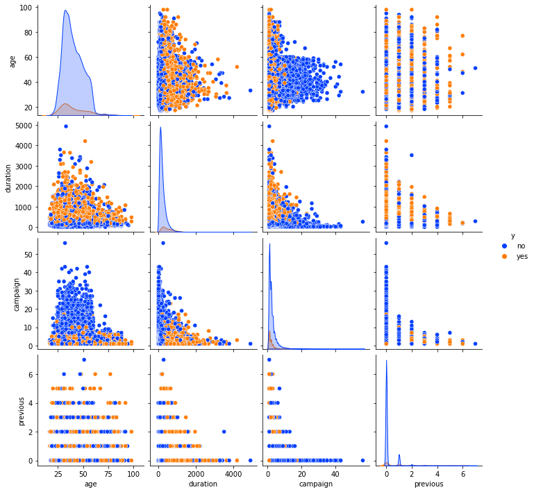
1# Arrays containing campaign and financial columns
2campaign_columns = ["age", "duration", "campaign", "previous"]
3financial_columns = [
4 "emp.var.rate",
5 "cons.price.idx",
6 "cons.conf.idx",
7 "euribor3m",
8]
9
10# Pairplot between campaign columns
11plot_data = dataset[campaign_columns + ["y"]]
12plt.figure(figsize=(10, 10))
13sns.pairplot(plot_data, hue="y", palette="bright")
14plt.savefig(f"{assets_path}/pairplot_campaign.png", format="png", dpi=300)
15
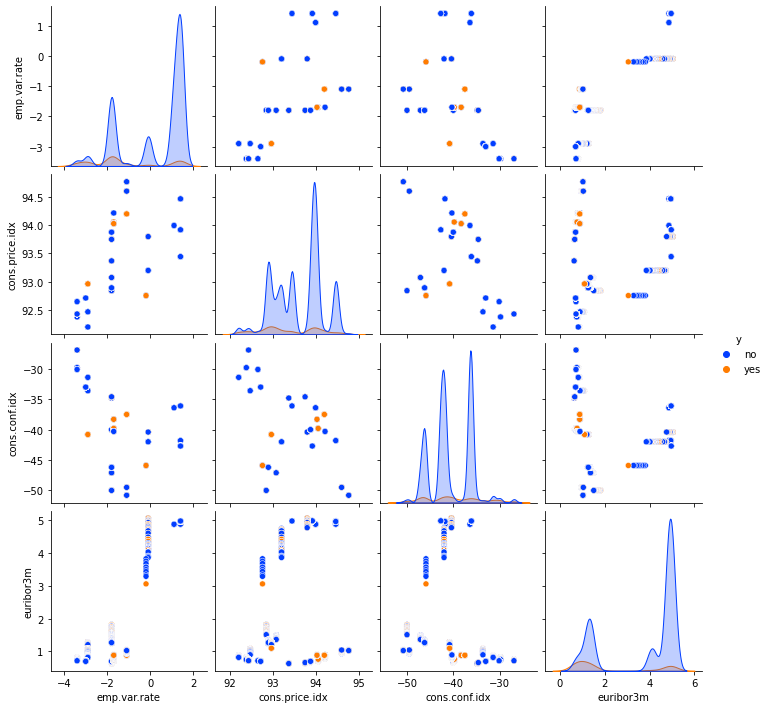
16# Pairplot between financial features
17plot_data = dataset[financial_columns + ["y"]]
18plt.figure(figsize=(10, 10))
19sns.pairplot(plot_data, hue="y", palette="bright")
20plt.savefig(f"{assets_path}/pairplot_financial.png", format="png", dpi=300)
<Figure size 720x720 with 0 Axes>
<Figure size 720x720 with 0 Axes>
Most of the successful marketing campaigns were with newly contacted customers. A substantial peak is present for customers who were contacted the second time, but without success.
For lower values for the 3-month interest rates (the euribor3m column), the number of successful marketing calls is larger than the number of unsuccessful ones. The inverse situation happens when interest rates are higher. A possible explanation for this phenomenon is customer optimism when interest rates are lower.
1# Mask for successful calls
2successful_calls = dataset.y == "yes"
3
4# Correlation matrix for successful calls
5plot_data = dataset[campaign_columns + financial_columns][successful_calls]
6successful_corr = plot_data.corr()
7successful_corr.style.background_gradient(cmap="coolwarm").set_precision(2)
| age | duration | campaign | previous | emp.var.rate | cons.price.idx | cons.conf.idx | euribor3m | |
|---|---|---|---|---|---|---|---|---|
| age | 1.00 | -0.06 | -0.01 | 0.07 | -0.08 | -0.02 | 0.14 | -0.09 |
| duration | -0.06 | 1.00 | 0.16 | -0.23 | 0.50 | 0.24 | -0.14 | 0.50 |
| campaign | -0.01 | 0.16 | 1.00 | -0.10 | 0.22 | 0.12 | -0.04 | 0.21 |
| previous | 0.07 | -0.23 | -0.10 | 1.00 | -0.28 | 0.09 | 0.13 | -0.39 |
| emp.var.rate | -0.08 | 0.50 | 0.22 | -0.28 | 1.00 | 0.66 | -0.27 | 0.93 |
| cons.price.idx | -0.02 | 0.24 | 0.12 | 0.09 | 0.66 | 1.00 | -0.33 | 0.41 |
| cons.conf.idx | 0.14 | -0.14 | -0.04 | 0.13 | -0.27 | -0.33 | 1.00 | -0.12 |
| euribor3m | -0.09 | 0.50 | 0.21 | -0.39 | 0.93 | 0.41 | -0.12 | 1.00 |
1# Correlation matrix for unsuccessful calls
2plot_data = dataset[campaign_columns + financial_columns][~successful_calls]
3unsuccessful_corr = plot_data.corr()
4unsuccessful_corr.style.background_gradient(cmap="coolwarm").set_precision(2)
| age | duration | campaign | previous | emp.var.rate | cons.price.idx | cons.conf.idx | euribor3m | |
|---|---|---|---|---|---|---|---|---|
| age | 1.00 | 0.00 | 0.01 | -0.00 | 0.03 | 0.01 | 0.12 | 0.04 |
| duration | 0.00 | 1.00 | -0.08 | -0.00 | 0.00 | 0.02 | 0.00 | 0.01 |
| campaign | 0.01 | -0.08 | 1.00 | -0.07 | 0.13 | 0.12 | -0.01 | 0.12 |
| previous | -0.00 | -0.00 | -0.07 | 1.00 | -0.42 | -0.27 | -0.14 | -0.44 |
| emp.var.rate | 0.03 | 0.00 | 0.13 | -0.42 | 1.00 | 0.80 | 0.32 | 0.98 |
| cons.price.idx | 0.01 | 0.02 | 0.12 | -0.27 | 0.80 | 1.00 | 0.15 | 0.73 |
| cons.conf.idx | 0.12 | 0.00 | -0.01 | -0.14 | 0.32 | 0.15 | 1.00 | 0.39 |
| euribor3m | 0.04 | 0.01 | 0.12 | -0.44 | 0.98 | 0.73 | 0.39 | 1.00 |
1# Plotting difference of successful - unsuccessful correlation matrices
2diff_corr = successful_corr - unsuccessful_corr
3diff_corr.style.background_gradient(cmap="coolwarm").set_precision(2)
| age | duration | campaign | previous | emp.var.rate | cons.price.idx | cons.conf.idx | euribor3m | |
|---|---|---|---|---|---|---|---|---|
| age | 0.00 | -0.06 | -0.02 | 0.08 | -0.11 | -0.04 | 0.02 | -0.13 |
| duration | -0.06 | 0.00 | 0.24 | -0.23 | 0.50 | 0.22 | -0.15 | 0.49 |
| campaign | -0.02 | 0.24 | 0.00 | -0.04 | 0.09 | -0.01 | -0.04 | 0.10 |
| previous | 0.08 | -0.23 | -0.04 | 0.00 | 0.14 | 0.36 | 0.27 | 0.05 |
| emp.var.rate | -0.11 | 0.50 | 0.09 | 0.14 | 0.00 | -0.14 | -0.59 | -0.05 |
| cons.price.idx | -0.04 | 0.22 | -0.01 | 0.36 | -0.14 | 0.00 | -0.48 | -0.32 |
| cons.conf.idx | 0.02 | -0.15 | -0.04 | 0.27 | -0.59 | -0.48 | 0.00 | -0.51 |
| euribor3m | -0.13 | 0.49 | 0.10 | 0.05 | -0.05 | -0.32 | -0.51 | 0.00 |
The correlation between euribor3m and emp.var.rate is very high (approximately 0.93 for successful and 0.98 for unsuccessful calls). The first one relates to the average interest rate at which European banks lend money to other banks with maturity of 3 months, while the second one relates to the employment variation, that is, the rate at which people are hired or fired in an economy.
Another column that is also highly correlated with the previous two is the Consumer Price Index (CPI) column: cons.price.idx. The consumer confidence index is negatively correlated with the three mentioned columns for successful customer calls, and positively correlated for unsuccessful ones. This means that when the overall economic sentiment is pessimistic, people are willing to accept the new banking products and vice versa.