Outliers and missing values

Importing libraries and packages

# Mathematical operations and data manipulation
import pandas as pd

# Visualisation
import seaborn as sns
import matplotlib.pyplot as plt

# Warnings
import warnings

warnings.filterwarnings("ignore")

%matplotlib inline

Set paths

# Path to datasets directory
data_path = "./datasets"
# Path to assets directory (for saving results to)
assets_path = "./assets"

Loading dataset

# load data
dataset = pd.read_csv(f"{data_path}/preprocessed_retail.csv")
dataset.head().T

	0	1	2	3	4
invoice	489434	489434	489434	489434	489434
stock_code	85048	79323P	79323W	22041	21232
desc	15CM CHRISTMAS GLASS BALL 20 LIGHTS	PINK CHERRY LIGHTS	WHITE CHERRY LIGHTS	RECORD FRAME 7" SINGLE SIZE	STRAWBERRY CERAMIC TRINKET BOX
quantity	12	12	12	48	24
date	01/12/2009 07:45	01/12/2009 07:45	01/12/2009 07:45	01/12/2009 07:45	01/12/2009 07:45
unit_price	6.95	6.75	6.75	2.1	1.25
cust_id	13085.0	13085.0	13085.0	13085.0	13085.0
country	United Kingdom	United Kingdom	United Kingdom	United Kingdom	United Kingdom

Outliers and missing values

dataset.isnull().sum().sort_values(ascending=False)

cust_id       107927
desc            2928
invoice            0
stock_code         0
quantity           0
date               0
unit_price         0
country            0
dtype: int64

dataset.describe()

	quantity	unit_price	cust_id
count	525461.000000	525461.000000	417534.000000
mean	10.337667	4.688834	15360.645478
std	107.424110	146.126914	1680.811316
min	-9600.000000	-53594.360000	12346.000000
25%	1.000000	1.250000	13983.000000
50%	3.000000	2.100000	15311.000000
75%	10.000000	4.210000	16799.000000
max	19152.000000	25111.090000	18287.000000

# How many instances in retail have 25111.09 (max) as their unit_price value?
dataset.loc[dataset["unit_price"] == 25111.090000]

	invoice	stock_code	desc	quantity	date	unit_price	cust_id	country
241824	C512770	M	Manual	-1	17/06/2010 16:52	25111.09	17399.0	United Kingdom
241827	512771	M	Manual	1	17/06/2010 16:53	25111.09	NaN	United Kingdom

# How many instances in retail have -53594.36 (min) as their unit_price value?
dataset.loc[dataset["unit_price"] == -53594.360000]

	invoice	stock_code	desc	quantity	date	unit_price	cust_id	country
179403	A506401	B	Adjust bad debt	1	29/04/2010 13:36	-53594.36	NaN	United Kingdom

Negative values for something like unit_price obviously don’t make sense.

# The total number of instances that have negative unit_price values
(dataset["unit_price"] <= 0).sum()

3690

This is only 0.7% of the total instances.

# The total number of instances that have negative quantity values
(dataset["quantity"] <= 0).sum()

12326

# How many instances have negative values for both the unit_price and
# quantity columns, and also have missing cust_id values?
(
    (dataset["unit_price"] <= 0)
    & (dataset["quantity"] <= 0)
    & (dataset["cust_id"].isnull())
).sum()

2121

0.4% of the total instances. Delete. Around 8000 instances with missing cust_ids will remain. Deleting those too. Storing the data with missing values in a DataFrame called null_dataset.

null_dataset = dataset[dataset.isnull().any(axis=1)]
null_dataset.head()

	invoice	stock_code	desc	quantity	date	unit_price	cust_id	country
263	489464	21733	85123a mixed	-96	01/12/2009 10:52	0.00	NaN	United Kingdom
283	489463	71477	short	-240	01/12/2009 10:52	0.00	NaN	United Kingdom
284	489467	85123A	21733 mixed	-192	01/12/2009 10:53	0.00	NaN	United Kingdom
470	489521	21646	NaN	-50	01/12/2009 11:44	0.00	NaN	United Kingdom
577	489525	85226C	BLUE PULL BACK RACING CAR	1	01/12/2009 11:49	0.55	NaN	United Kingdom

dataset.to_csv(f"{data_path}/null_retail.csv", index=False)

new_dataset = dataset.dropna()

new_dataset = new_dataset[
    (new_dataset["unit_price"] > 0) & (new_dataset["quantity"] > 0)
]
new_dataset.describe()

	quantity	unit_price	cust_id
count	407664.000000	407664.000000	407664.000000
mean	13.585585	3.294438	15368.592598
std	96.840747	34.757965	1679.762138
min	1.000000	0.001000	12346.000000
25%	2.000000	1.250000	13997.000000
50%	5.000000	1.950000	15321.000000
75%	12.000000	3.750000	16812.000000
max	19152.000000	10953.500000	18287.000000

# Boxplot for the unit_price column
plt.subplots(figsize=(12, 6))
up = sns.boxplot(new_dataset.unit_price)

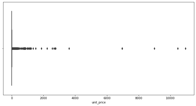
Most are between 0-4000. There are four data points beyond 6000. Keeping only those below 6000.

new_dataset = new_dataset[new_dataset.unit_price < 6000]
new_dataset.describe()

	quantity	unit_price	cust_id
count	407659.000000	407659.000000	407659.000000
mean	13.585740	3.185750	15368.593562
std	96.841331	14.494341	1679.761725
min	1.000000	0.001000	12346.000000
25%	2.000000	1.250000	13997.000000
50%	5.000000	1.950000	15321.000000
75%	12.000000	3.750000	16812.000000
max	19152.000000	3610.500000	18287.000000

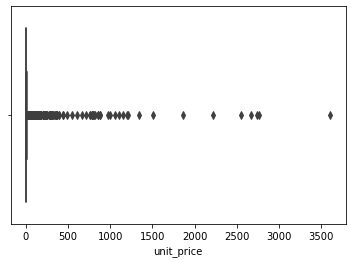
# Boxplot of the new unit_price column to see the changes
up_new = sns.boxplot(new_dataset.unit_price)

# Boxplot of the new quantity column to see the changes
plt.subplots(figsize=(12, 6))
q = sns.boxplot(new_dataset.quantity)

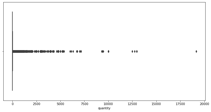
One anomaly here between 17,500 and 20,000. Also, the majority of the data points are between 1 and 7,500, with a few ranging from 7,500 to around 13,500. Deleting.

new_dataset = new_dataset[new_dataset.quantity < 15000]
new_dataset.describe()

	quantity	unit_price	cust_id
count	407658.000000	407658.000000	407658.000000
mean	13.538792	3.185757	15368.597160
std	92.085647	14.494358	1679.762214
min	1.000000	0.001000	12346.000000
25%	2.000000	1.250000	13997.000000
50%	5.000000	1.950000	15321.000000
75%	12.000000	3.750000	16812.000000
max	12960.000000	3610.500000	18287.000000

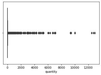
q_new = sns.boxplot(new_dataset.quantity)

dataset = new_dataset
dataset.head()

	invoice	stock_code	desc	quantity	date	unit_price	cust_id	country
0	489434	85048	15CM CHRISTMAS GLASS BALL 20 LIGHTS	12	01/12/2009 07:45	6.95	13085.0	United Kingdom
1	489434	79323P	PINK CHERRY LIGHTS	12	01/12/2009 07:45	6.75	13085.0	United Kingdom
2	489434	79323W	WHITE CHERRY LIGHTS	12	01/12/2009 07:45	6.75	13085.0	United Kingdom
3	489434	22041	RECORD FRAME 7" SINGLE SIZE	48	01/12/2009 07:45	2.10	13085.0	United Kingdom
4	489434	21232	STRAWBERRY CERAMIC TRINKET BOX	24	01/12/2009 07:45	1.25	13085.0	United Kingdom

dataset.to_csv(f"{data_path}/cleaned_retail.csv", index=False)