

Exploratory data analysis#
Uncovering underlying data structures.
Importing libraries and packages#
 1# Mathematical operations and data manipulation
 2import pandas as pd
 3
 4# Plotting
 5import seaborn as sns
 6import matplotlib.pyplot as plt
 7
 8# Warnings
 9import warnings
10
11warnings.filterwarnings("ignore")
12
13%matplotlib inline
Set paths#
1# Path to datasets directory
2data_path = "./datasets"
3# Path to assets directory (for saving results to)
4assets_path = "./assets"
Loading dataset#
1# load data
2dataset = pd.read_csv(f"{data_path}/preprocessed_default_credit.csv")
3dataset.head().T
| 0 | 1 | 2 | 3 | 4 | |
|---|---|---|---|---|---|
| ID | 1 | 2 | 3 | 4 | 5 |
| LIMIT_BAL | 20000 | 120000 | 90000 | 50000 | 50000 |
| SEX | 2 | 2 | 2 | 2 | 1 |
| EDUCATION | 2 | 2 | 2 | 2 | 2 |
| MARRIAGE | 1 | 2 | 2 | 1 | 1 |
| AGE | 24 | 26 | 34 | 37 | 57 |
| PAY_1 | 2 | -1 | 0 | 0 | -1 |
| PAY_2 | 2 | 2 | 0 | 0 | 0 |
| PAY_3 | -1 | 0 | 0 | 0 | -1 |
| PAY_4 | -1 | 0 | 0 | 0 | 0 |
| PAY_5 | -2 | 0 | 0 | 0 | 0 |
| PAY_6 | -2 | 2 | 0 | 0 | 0 |
| BILL_AMT1 | 3913 | 2682 | 29239 | 46990 | 8617 |
| BILL_AMT2 | 3102 | 1725 | 14027 | 48233 | 5670 |
| BILL_AMT3 | 689 | 2682 | 13559 | 49291 | 35835 |
| BILL_AMT4 | 0 | 3272 | 14331 | 28314 | 20940 |
| BILL_AMT5 | 0 | 3455 | 14948 | 28959 | 19146 |
| BILL_AMT6 | 0 | 3261 | 15549 | 29547 | 19131 |
| PAY_AMT1 | 0 | 0 | 1518 | 2000 | 2000 |
| PAY_AMT2 | 689 | 1000 | 1500 | 2019 | 36681 |
| PAY_AMT3 | 0 | 1000 | 1000 | 1200 | 10000 |
| PAY_AMT4 | 0 | 1000 | 1000 | 1100 | 9000 |
| PAY_AMT5 | 0 | 0 | 1000 | 1069 | 689 |
| PAY_AMT6 | 0 | 2000 | 5000 | 1000 | 679 |
| DEFAULT | 1 | 1 | 0 | 0 | 0 |
Exploring dataset#
1# Printing dimensionality of the data, columns, types and missing values
2print(f"Data dimension: {dataset.shape}")
3for col in dataset.columns:
4    print(
5        f"Column: {col:35} | "
6        f"type: {str(dataset[col].dtype):7} | "
7        f"missing values: {dataset[col].isna().sum():3d}"
8    )
Data dimension: (30000, 25)
Column: ID                                  | type: int64   | missing values:   0
Column: LIMIT_BAL                           | type: int64   | missing values:   0
Column: SEX                                 | type: int64   | missing values:   0
Column: EDUCATION                           | type: int64   | missing values:   0
Column: MARRIAGE                            | type: int64   | missing values:   0
Column: AGE                                 | type: int64   | missing values:   0
Column: PAY_1                               | type: int64   | missing values:   0
Column: PAY_2                               | type: int64   | missing values:   0
Column: PAY_3                               | type: int64   | missing values:   0
Column: PAY_4                               | type: int64   | missing values:   0
Column: PAY_5                               | type: int64   | missing values:   0
Column: PAY_6                               | type: int64   | missing values:   0
Column: BILL_AMT1                           | type: int64   | missing values:   0
Column: BILL_AMT2                           | type: int64   | missing values:   0
Column: BILL_AMT3                           | type: int64   | missing values:   0
Column: BILL_AMT4                           | type: int64   | missing values:   0
Column: BILL_AMT5                           | type: int64   | missing values:   0
Column: BILL_AMT6                           | type: int64   | missing values:   0
Column: PAY_AMT1                            | type: int64   | missing values:   0
Column: PAY_AMT2                            | type: int64   | missing values:   0
Column: PAY_AMT3                            | type: int64   | missing values:   0
Column: PAY_AMT4                            | type: int64   | missing values:   0
Column: PAY_AMT5                            | type: int64   | missing values:   0
Column: PAY_AMT6                            | type: int64   | missing values:   0
Column: DEFAULT                             | type: int64   | missing values:   0
1# Computing statistics on numerical features
2dataset.describe().T
| count | mean | std | min | 25% | 50% | 75% | max | |
|---|---|---|---|---|---|---|---|---|
| ID | 30000.0 | 15000.500000 | 8660.398374 | 1.0 | 7500.75 | 15000.5 | 22500.25 | 30000.0 |
| LIMIT_BAL | 30000.0 | 167484.322667 | 129747.661567 | 10000.0 | 50000.00 | 140000.0 | 240000.00 | 1000000.0 |
| SEX | 30000.0 | 1.603733 | 0.489129 | 1.0 | 1.00 | 2.0 | 2.00 | 2.0 |
| EDUCATION | 30000.0 | 1.842267 | 0.744494 | 1.0 | 1.00 | 2.0 | 2.00 | 4.0 |
| MARRIAGE | 30000.0 | 1.555467 | 0.518137 | 1.0 | 1.00 | 2.0 | 2.00 | 3.0 |
| AGE | 30000.0 | 35.485500 | 9.217904 | 21.0 | 28.00 | 34.0 | 41.00 | 79.0 |
| PAY_1 | 30000.0 | -0.016700 | 1.123802 | -2.0 | -1.00 | 0.0 | 0.00 | 8.0 |
| PAY_2 | 30000.0 | -0.133767 | 1.197186 | -2.0 | -1.00 | 0.0 | 0.00 | 8.0 |
| PAY_3 | 30000.0 | -0.166200 | 1.196868 | -2.0 | -1.00 | 0.0 | 0.00 | 8.0 |
| PAY_4 | 30000.0 | -0.220667 | 1.169139 | -2.0 | -1.00 | 0.0 | 0.00 | 8.0 |
| PAY_5 | 30000.0 | -0.266200 | 1.133187 | -2.0 | -1.00 | 0.0 | 0.00 | 8.0 |
| PAY_6 | 30000.0 | -0.291100 | 1.149988 | -2.0 | -1.00 | 0.0 | 0.00 | 8.0 |
| BILL_AMT1 | 30000.0 | 51223.330900 | 73635.860576 | -165580.0 | 3558.75 | 22381.5 | 67091.00 | 964511.0 |
| BILL_AMT2 | 30000.0 | 49179.075167 | 71173.768783 | -69777.0 | 2984.75 | 21200.0 | 64006.25 | 983931.0 |
| BILL_AMT3 | 30000.0 | 47013.154800 | 69349.387427 | -157264.0 | 2666.25 | 20088.5 | 60164.75 | 1664089.0 |
| BILL_AMT4 | 30000.0 | 43262.948967 | 64332.856134 | -170000.0 | 2326.75 | 19052.0 | 54506.00 | 891586.0 |
| BILL_AMT5 | 30000.0 | 40311.400967 | 60797.155770 | -81334.0 | 1763.00 | 18104.5 | 50190.50 | 927171.0 |
| BILL_AMT6 | 30000.0 | 38871.760400 | 59554.107537 | -339603.0 | 1256.00 | 17071.0 | 49198.25 | 961664.0 |
| PAY_AMT1 | 30000.0 | 5663.580500 | 16563.280354 | 0.0 | 1000.00 | 2100.0 | 5006.00 | 873552.0 |
| PAY_AMT2 | 30000.0 | 5921.163500 | 23040.870402 | 0.0 | 833.00 | 2009.0 | 5000.00 | 1684259.0 |
| PAY_AMT3 | 30000.0 | 5225.681500 | 17606.961470 | 0.0 | 390.00 | 1800.0 | 4505.00 | 896040.0 |
| PAY_AMT4 | 30000.0 | 4826.076867 | 15666.159744 | 0.0 | 296.00 | 1500.0 | 4013.25 | 621000.0 |
| PAY_AMT5 | 30000.0 | 4799.387633 | 15278.305679 | 0.0 | 252.50 | 1500.0 | 4031.50 | 426529.0 |
| PAY_AMT6 | 30000.0 | 5215.502567 | 17777.465775 | 0.0 | 117.75 | 1500.0 | 4000.00 | 528666.0 |
| DEFAULT | 30000.0 | 0.221200 | 0.415062 | 0.0 | 0.00 | 0.0 | 0.00 | 1.0 |
Univariate analysis#
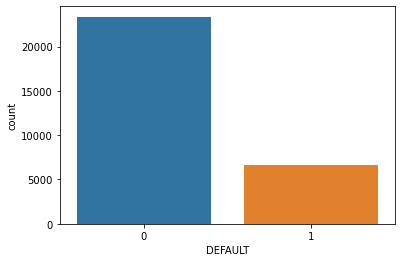
1# Count of the DEFAULT column
2sns.countplot(x="DEFAULT", data=dataset)
<AxesSubplot:xlabel='DEFAULT', ylabel='count'>
1# Distribution of the DEFAULT column, that is, the count of
2# defaults versus non-defaults
3print(dataset["DEFAULT"].value_counts())
4print()
5print(dataset["DEFAULT"].value_counts(normalize=True))
0    23364
1     6636
Name: DEFAULT, dtype: int64

0    0.7788
1    0.2212
Name: DEFAULT, dtype: float64
Around 6636 customers have defaulted out of 30000 people, which is around 22%.
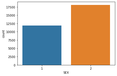
1# The SEX column
2sns.countplot(x="SEX", data=dataset)
<AxesSubplot:xlabel='SEX', ylabel='count'>
1# Calculation exact number of each visitor type
2print(dataset["SEX"].value_counts())
3print()
4print(dataset["SEX"].value_counts(normalize=True))
2    18112
1    11888
Name: SEX, dtype: int64

2    0.603733
1    0.396267
Name: SEX, dtype: float64
There are a total of 18112 females and 11888 males in the given dataset.
1# EDUCATION column
2sns.countplot(x="EDUCATION", data=dataset)
<AxesSubplot:xlabel='EDUCATION', ylabel='count'>
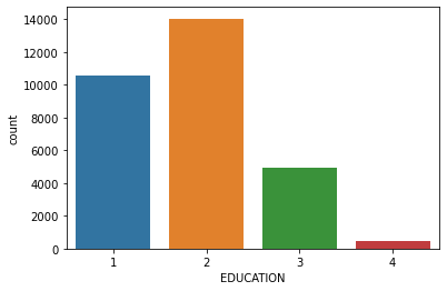
1print(dataset["EDUCATION"].value_counts())
2print()
3print(dataset["EDUCATION"].value_counts(normalize=True))
2    14030
1    10585
3     4917
4      468
Name: EDUCATION, dtype: int64

2    0.467667
1    0.352833
3    0.163900
4    0.015600
Name: EDUCATION, dtype: float64
Most customers either went to graduate school or university.
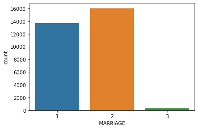
1# MARRIAGE column
2sns.countplot(x="MARRIAGE", data=dataset)
<AxesSubplot:xlabel='MARRIAGE', ylabel='count'>
1# Count of each subcategory in the weekend column
2print(dataset["MARRIAGE"].value_counts())
3print()
4print(dataset["MARRIAGE"].value_counts(normalize=True))
2    16018
1    13659
3      323
Name: MARRIAGE, dtype: int64

2    0.533933
1    0.455300
3    0.010767
Name: MARRIAGE, dtype: float64
Dataset has a high number of people who are single (unmarried) and people who are married.
Bivariate analysis#
1# The SEX column versus the DEFAULT column
2sns.set(rc={"figure.figsize": (15, 10)})
3edu = sns.countplot(x="SEX", hue="DEFAULT", data=dataset)
4edu.set_xticklabels(["Male", "Female"])
5plt.show()
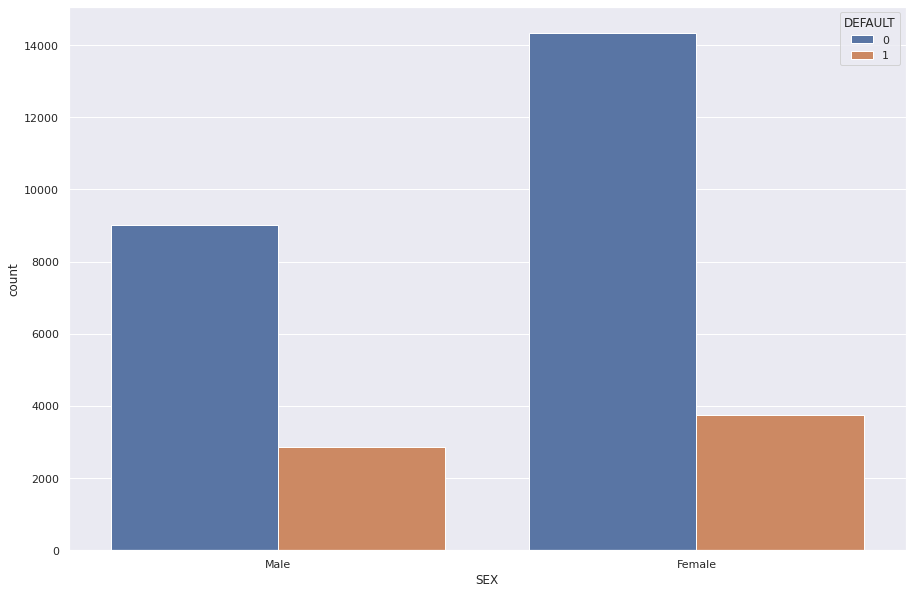
Females seem to have defaulted more than males.
1# Cross-tabulation
2pd.crosstab(dataset.SEX, dataset.DEFAULT, normalize="index", margins=True)
| DEFAULT | 0 | 1 |
|---|---|---|
| SEX | ||
| 1 | 0.758328 | 0.241672 |
| 2 | 0.792237 | 0.207763 |
| All | 0.778800 | 0.221200 |
The cross tabulation shows that sround 24% of male customers have defaulted and around 20% of female customers have defaulted.
Relationship between the DEFAULT Column and the EDUCATION and MARRIAGE Columns#
1sns.set(rc={"figure.figsize": (15, 10)})
2edu = sns.countplot(x="EDUCATION", hue="DEFAULT", data=dataset)
3edu.set_xticklabels(["Graduate School", "University", "High School", "Other"])
4plt.show()
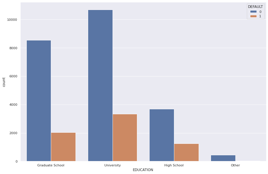
1# Determining which subcategory has a higher default percentage
2# with cross-tabulation
3pd.crosstab(dataset.EDUCATION, dataset.DEFAULT, normalize="index")
| DEFAULT | 0 | 1 |
|---|---|---|
| EDUCATION | ||
| 1 | 0.807652 | 0.192348 |
| 2 | 0.762651 | 0.237349 |
| 3 | 0.748424 | 0.251576 |
| 4 | 0.929487 | 0.070513 |
1# Relationship between the MARRIAGE and DEFAULT columns
2sns.set(rc={"figure.figsize": (12, 10)})
3marriage = sns.countplot(x="MARRIAGE", hue="DEFAULT", data=dataset)
4marriage.set_xticklabels(["Married", "Single", "Other"])
5plt.show()
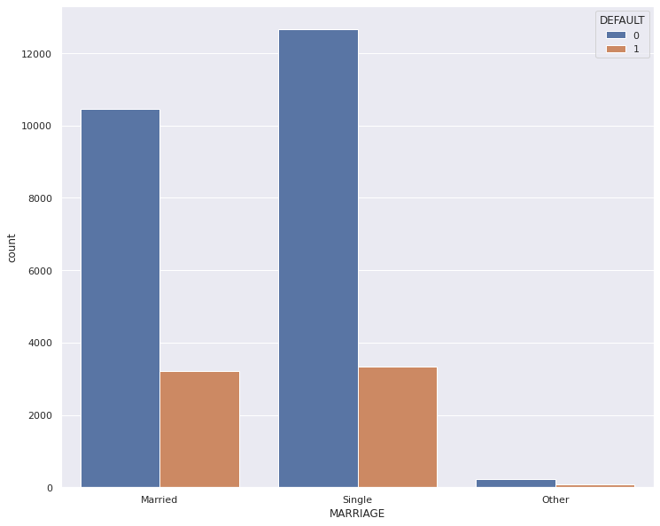
1# Percentage of married/single/other people which have defaulted
2pd.crosstab(dataset.MARRIAGE, dataset.DEFAULT, normalize="index", margins=True)
| DEFAULT | 0 | 1 |
|---|---|---|
| MARRIAGE | ||
| 1 | 0.765283 | 0.234717 |
| 2 | 0.791110 | 0.208890 |
| 3 | 0.739938 | 0.260062 |
| All | 0.778800 | 0.221200 |
Relationships#
1# Bounce Rate versus Exit Rate
2pd.crosstab(dataset.AGE, dataset.DEFAULT)
| DEFAULT | 0 | 1 |
|---|---|---|
| AGE | ||
| 21 | 53 | 14 |
| 22 | 391 | 169 |
| 23 | 684 | 247 |
| 24 | 827 | 300 |
| 25 | 884 | 302 |
| 26 | 1003 | 253 |
| 27 | 1164 | 313 |
| 28 | 1123 | 286 |
| 29 | 1292 | 313 |
| 30 | 1121 | 274 |
| 31 | 988 | 229 |
| 32 | 933 | 225 |
| 33 | 931 | 215 |
| 34 | 931 | 231 |
| 35 | 887 | 226 |
| 36 | 854 | 254 |
| 37 | 812 | 229 |
| 38 | 750 | 194 |
| 39 | 755 | 199 |
| 40 | 683 | 187 |
| 41 | 639 | 185 |
| 42 | 609 | 185 |
| 43 | 520 | 150 |
| 44 | 538 | 162 |
| 45 | 501 | 116 |
| 46 | 413 | 157 |
| 47 | 381 | 120 |
| 48 | 362 | 104 |
| 49 | 333 | 119 |
| 50 | 310 | 101 |
| 51 | 252 | 88 |
| 52 | 226 | 78 |
| 53 | 251 | 74 |
| 54 | 191 | 56 |
| 55 | 152 | 57 |
| 56 | 129 | 49 |
| 57 | 95 | 27 |
| 58 | 91 | 31 |
| 59 | 62 | 21 |
| 60 | 44 | 23 |
| 61 | 35 | 21 |
| 62 | 37 | 7 |
| 63 | 23 | 8 |
| 64 | 22 | 9 |
| 65 | 19 | 5 |
| 66 | 18 | 7 |
| 67 | 11 | 5 |
| 68 | 4 | 1 |
| 69 | 12 | 3 |
| 70 | 8 | 2 |
| 71 | 3 | 0 |
| 72 | 2 | 1 |
| 73 | 1 | 3 |
| 74 | 1 | 0 |
| 75 | 2 | 1 |
| 79 | 1 | 0 |
1pd.crosstab(dataset.AGE, dataset.DEFAULT, normalize="index", margins=True)
| DEFAULT | 0 | 1 |
|---|---|---|
| AGE | ||
| 21 | 0.791045 | 0.208955 |
| 22 | 0.698214 | 0.301786 |
| 23 | 0.734694 | 0.265306 |
| 24 | 0.733807 | 0.266193 |
| 25 | 0.745363 | 0.254637 |
| 26 | 0.798567 | 0.201433 |
| 27 | 0.788084 | 0.211916 |
| 28 | 0.797019 | 0.202981 |
| 29 | 0.804984 | 0.195016 |
| 30 | 0.803584 | 0.196416 |
| 31 | 0.811832 | 0.188168 |
| 32 | 0.805699 | 0.194301 |
| 33 | 0.812391 | 0.187609 |
| 34 | 0.801205 | 0.198795 |
| 35 | 0.796945 | 0.203055 |
| 36 | 0.770758 | 0.229242 |
| 37 | 0.780019 | 0.219981 |
| 38 | 0.794492 | 0.205508 |
| 39 | 0.791405 | 0.208595 |
| 40 | 0.785057 | 0.214943 |
| 41 | 0.775485 | 0.224515 |
| 42 | 0.767003 | 0.232997 |
| 43 | 0.776119 | 0.223881 |
| 44 | 0.768571 | 0.231429 |
| 45 | 0.811994 | 0.188006 |
| 46 | 0.724561 | 0.275439 |
| 47 | 0.760479 | 0.239521 |
| 48 | 0.776824 | 0.223176 |
| 49 | 0.736726 | 0.263274 |
| 50 | 0.754258 | 0.245742 |
| 51 | 0.741176 | 0.258824 |
| 52 | 0.743421 | 0.256579 |
| 53 | 0.772308 | 0.227692 |
| 54 | 0.773279 | 0.226721 |
| 55 | 0.727273 | 0.272727 |
| 56 | 0.724719 | 0.275281 |
| 57 | 0.778689 | 0.221311 |
| 58 | 0.745902 | 0.254098 |
| 59 | 0.746988 | 0.253012 |
| 60 | 0.656716 | 0.343284 |
| 61 | 0.625000 | 0.375000 |
| 62 | 0.840909 | 0.159091 |
| 63 | 0.741935 | 0.258065 |
| 64 | 0.709677 | 0.290323 |
| 65 | 0.791667 | 0.208333 |
| 66 | 0.720000 | 0.280000 |
| 67 | 0.687500 | 0.312500 |
| 68 | 0.800000 | 0.200000 |
| 69 | 0.800000 | 0.200000 |
| 70 | 0.800000 | 0.200000 |
| 71 | 1.000000 | 0.000000 |
| 72 | 0.666667 | 0.333333 |
| 73 | 0.250000 | 0.750000 |
| 74 | 1.000000 | 0.000000 |
| 75 | 0.666667 | 0.333333 |
| 79 | 1.000000 | 0.000000 |
| All | 0.778800 | 0.221200 |