Data analysis

Importing libraries and packages

# Mathematical operations and data manipulation
import numpy as np
import pandas as pd

# Plotting
import seaborn as sns
import matplotlib.pyplot as plt

# Warnings
import warnings

warnings.filterwarnings("ignore")

%matplotlib inline

Set paths

# Path to datasets directory
data_path = "./datasets"
# Path to assets directory (for saving results to)
assets_path = "./assets"

Loading dataset

# load data
dataset = pd.read_csv(f"{data_path}/cleaned_airquality.csv")
dataset.head().T

	0	1	2	3	4
year	2013	2013	2013	2013	2013
month	3	3	3	3	3
day	1	1	1	1	1
hour	0	1	2	3	4
PM25	4.0	8.0	7.0	6.0	3.0
PM10	4.0	8.0	7.0	6.0	3.0
SO2	4.0	4.0	5.0	11.0	12.0
NO2	7.0	7.0	10.0	11.0	12.0
CO	300.0	300.0	300.0	300.0	300.0
O3	77.0	77.0	73.0	72.0	72.0
TEMP	-0.7	-1.1	-1.1	-1.4	-2.0
PRES	1023.0	1023.2	1023.5	1024.5	1025.2
DEWP	-18.8	-18.2	-18.2	-19.4	-19.5
RAIN	0.0	0.0	0.0	0.0	0.0
wd	NNW	N	NNW	NW	N
WSPM	4.4	4.7	5.6	3.1	2.0
station	Aotizhongxin	Aotizhongxin	Aotizhongxin	Aotizhongxin	Aotizhongxin

Data analysis

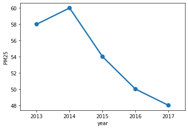
The Concentration of PM25 and PM10 per Year

year_pm25 = (
    dataset[["PM25", "year", "station"]]
    .groupby(["year"])
    .median()
    .reset_index()
    .sort_values(by="year", ascending=False)
)

year_pm25

	year	PM25
4	2017	48.0
3	2016	50.0
2	2015	54.0
1	2014	60.0
0	2013	58.0

sns.pointplot(x="year", y="PM25", data=year_pm25)

<AxesSubplot:xlabel='year', ylabel='PM25'>

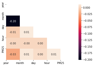
Checking for Correlations between Features

corr = dataset.corr()
mask = np.zeros_like(corr, dtype=np.bool)
mask[np.triu_indices_from(mask)] = True
sns.heatmap(corr, annot=True, fmt=".2f", mask=mask)
plt.xticks(range(len(corr.columns)), corr.columns)
plt.yticks(range(len(corr.columns)), corr.columns)
plt.show()