Exploratory data analysis

Uncovering underlying data structures.

Importing libraries and packages

# Mathematical operations and data manipulation
import pandas as pd

# Plotting
import seaborn as sns
import matplotlib.pyplot as plt

# Warnings
import warnings

warnings.filterwarnings("ignore")

%matplotlib inline

Set paths

# Path to datasets directory
data_path = "./datasets"
# Path to assets directory (for saving results to)
assets_path = "./assets"

Loading dataset

# load data
dataset = pd.read_csv(f"{data_path}/online_shoppers_intention.csv")
dataset.head().T

	0	1	2	3	4
Administrative	0	0	0	0	0
Administrative_Duration	0.0	0.0	0.0	0.0	0.0
Informational	0	0	0	0	0
Informational_Duration	0.0	0.0	0.0	0.0	0.0
ProductRelated	1	2	1	2	10
ProductRelated_Duration	0.0	64.0	0.0	2.666667	627.5
BounceRates	0.2	0.0	0.2	0.05	0.02
ExitRates	0.2	0.1	0.2	0.14	0.05
PageValues	0.0	0.0	0.0	0.0	0.0
SpecialDay	0.0	0.0	0.0	0.0	0.0
Month	Feb	Feb	Feb	Feb	Feb
OperatingSystems	1	2	4	3	3
Browser	1	2	1	2	3
Region	1	1	9	2	1
TrafficType	1	2	3	4	4
VisitorType	Returning_Visitor	Returning_Visitor	Returning_Visitor	Returning_Visitor	Returning_Visitor
Weekend	False	False	False	False	True
Revenue	False	False	False	False	False

Exploring dataset

# Printing dimensionality of the data, columns, types and missing values
print(f"Data dimension: {dataset.shape}")
for col in dataset.columns:
    print(
        f"Column: {col:35} | "
        f"type: {str(dataset[col].dtype):7} | "
        f"missing values: {dataset[col].isna().sum():3d}"
    )

Data dimension: (12330, 18)
Column: Administrative                      | type: int64   | missing values:   0
Column: Administrative_Duration             | type: float64 | missing values:   0
Column: Informational                       | type: int64   | missing values:   0
Column: Informational_Duration              | type: float64 | missing values:   0
Column: ProductRelated                      | type: int64   | missing values:   0
Column: ProductRelated_Duration             | type: float64 | missing values:   0
Column: BounceRates                         | type: float64 | missing values:   0
Column: ExitRates                           | type: float64 | missing values:   0
Column: PageValues                          | type: float64 | missing values:   0
Column: SpecialDay                          | type: float64 | missing values:   0
Column: Month                               | type: object  | missing values:   0
Column: OperatingSystems                    | type: int64   | missing values:   0
Column: Browser                             | type: int64   | missing values:   0
Column: Region                              | type: int64   | missing values:   0
Column: TrafficType                         | type: int64   | missing values:   0
Column: VisitorType                         | type: object  | missing values:   0
Column: Weekend                             | type: bool    | missing values:   0
Column: Revenue                             | type: bool    | missing values:   0

# Computing statistics on numerical features
dataset.describe().T

	count	mean	std	min	25%	50%	75%	max
Administrative	12330.0	2.315166	3.321784	0.0	0.000000	1.000000	4.000000	27.000000
Administrative_Duration	12330.0	80.818611	176.779107	0.0	0.000000	7.500000	93.256250	3398.750000
Informational	12330.0	0.503569	1.270156	0.0	0.000000	0.000000	0.000000	24.000000
Informational_Duration	12330.0	34.472398	140.749294	0.0	0.000000	0.000000	0.000000	2549.375000
ProductRelated	12330.0	31.731468	44.475503	0.0	7.000000	18.000000	38.000000	705.000000
ProductRelated_Duration	12330.0	1194.746220	1913.669288	0.0	184.137500	598.936905	1464.157214	63973.522230
BounceRates	12330.0	0.022191	0.048488	0.0	0.000000	0.003112	0.016813	0.200000
ExitRates	12330.0	0.043073	0.048597	0.0	0.014286	0.025156	0.050000	0.200000
PageValues	12330.0	5.889258	18.568437	0.0	0.000000	0.000000	0.000000	361.763742
SpecialDay	12330.0	0.061427	0.198917	0.0	0.000000	0.000000	0.000000	1.000000
OperatingSystems	12330.0	2.124006	0.911325	1.0	2.000000	2.000000	3.000000	8.000000
Browser	12330.0	2.357097	1.717277	1.0	2.000000	2.000000	2.000000	13.000000
Region	12330.0	3.147364	2.401591	1.0	1.000000	3.000000	4.000000	9.000000
TrafficType	12330.0	4.069586	4.025169	1.0	2.000000	2.000000	4.000000	20.000000

Univariate analysis

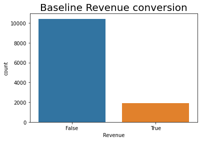
# Baseline Conversion Rate from the Revenue Column
sns.countplot(dataset["Revenue"])
plt.title("Baseline Revenue conversion", fontsize=20)
plt.show()

print(dataset["Revenue"].value_counts())
print()
print(dataset["Revenue"].value_counts(normalize=True))

False    10422
True      1908
Name: Revenue, dtype: int64

False    0.845255
True     0.154745
Name: Revenue, dtype: float64

The baseline conversion rate of online visitors versus overall visitors is a ratio between the total number of online sessions that led to a purchase divided by the total number of sessions.

print(1908 / 12330 * 100)

15.474452554744525

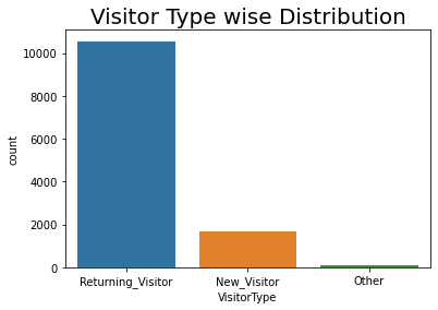
# Visitor-Wise Distribution
sns.countplot(dataset["VisitorType"])
plt.title("Visitor Type wise Distribution", fontsize=20)
plt.show()

# Calculation exact number of each visitor type
print(dataset["VisitorType"].value_counts())
print()
print(dataset["VisitorType"].value_counts(normalize=True))

Returning_Visitor    10551
New_Visitor           1694
Other                   85
Name: VisitorType, dtype: int64

Returning_Visitor    0.855718
New_Visitor          0.137388
Other                0.006894
Name: VisitorType, dtype: float64

The number of returning customers is higher than that of new visitors.

# Traffic-Wise Distribution
sns.countplot(dataset["TrafficType"])
plt.title("Traffic Type wise Distribution", fontsize=20)
plt.show()

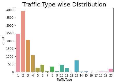
print(dataset["TrafficType"].value_counts(normalize=True))

2     0.317356
1     0.198783
3     0.166423
4     0.086699
13    0.059854
10    0.036496
6     0.036010
8     0.027818
5     0.021087
11    0.020032
20    0.016058
9     0.003406
7     0.003244
15    0.003082
19    0.001379
14    0.001054
18    0.000811
16    0.000243
12    0.000081
17    0.000081
Name: TrafficType, dtype: float64

Sources 2, 1, 3, and 4 account for the majority of our web traffic.

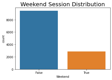
# Distribution of Customers Session on the Website
sns.countplot(dataset["Weekend"])
plt.title("Weekend Session Distribution", fontsize=20)
plt.show()

# Count of each subcategory in the weekend column
print(dataset["Weekend"].value_counts())
print()
print(dataset["Weekend"].value_counts(normalize=True))

False    9462
True     2868
Name: Weekend, dtype: int64

False    0.767397
True     0.232603
Name: Weekend, dtype: float64

More visitors visit during weekdays than weekend days.

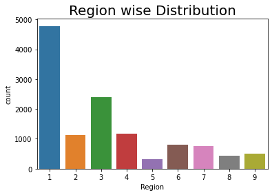
# Region-Wise Distribution
sns.countplot(dataset["Region"])
plt.title("Region wise Distribution", fontsize=20)
plt.show()

print(dataset["Region"].value_counts())
print()
print(dataset["Region"].value_counts(normalize=True))

1    4780
3    2403
4    1182
2    1136
6     805
7     761
9     511
8     434
5     318
Name: Region, dtype: int64

1    0.387672
3    0.194891
4    0.095864
2    0.092133
6    0.065288
7    0.061719
9    0.041444
8    0.035199
5    0.025791
Name: Region, dtype: float64

Regions 1 and 3 account for 50% of online sessions.

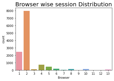
# Browser and OS Distribution of Customers
sns.countplot(dataset["Browser"])
plt.title("Browser wise session Distribution", fontsize=20)
plt.show()

print(dataset["Browser"].value_counts())
print()
print(dataset["Browser"].value_counts(normalize=True))

2     7961
1     2462
4      736
5      467
6      174
10     163
8      135
3      105
13      61
7       49
12      10
11       6
9        1
Name: Browser, dtype: int64

2     0.645661
1     0.199676
4     0.059692
5     0.037875
6     0.014112
10    0.013220
8     0.010949
3     0.008516
13    0.004947
7     0.003974
12    0.000811
11    0.000487
9     0.000081
Name: Browser, dtype: float64

sns.countplot(dataset["OperatingSystems"])
plt.title("OS wise session Distribution", fontsize=20)
plt.show()

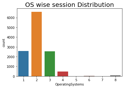
print(dataset["OperatingSystems"].value_counts())
print()
print(dataset["OperatingSystems"].value_counts(normalize=True))

2    6601
1    2585
3    2555
4     478
8      79
6      19
7       7
5       6
Name: OperatingSystems, dtype: int64

2    0.535361
1    0.209651
3    0.207218
4    0.038767
8    0.006407
6    0.001541
7    0.000568
5    0.000487
Name: OperatingSystems, dtype: float64

# Administrative Pageview Distribution
sns.countplot(dataset["Administrative"])
plt.title("Administrative Pageview Distribution", fontsize=16)
plt.show()

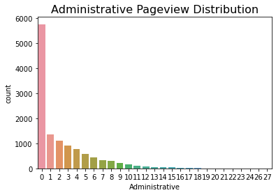
Users tend to visit page 0 the most often.

# Information Pageview Distribution
sns.countplot(dataset["Informational"])
plt.title("Information Pageview Distribution", fontsize=16)
plt.show()

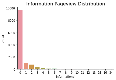
# Percentage count for each information page
print(dataset["Informational"].value_counts(normalize=True))

0     0.786618
1     0.084428
2     0.059043
3     0.030819
4     0.018005
5     0.008029
6     0.006326
7     0.002920
9     0.001217
8     0.001135
10    0.000568
12    0.000406
14    0.000162
16    0.000081
11    0.000081
24    0.000081
13    0.000081
Name: Informational, dtype: float64

79% of users are visiting pages 0 and 1.

# Special Day Session Distribution
sns.countplot(dataset["SpecialDay"])
plt.title("Special Day session Distribution", fontsize=16)
plt.show()

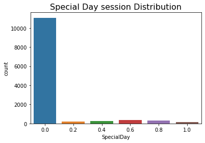
# Percentage distribution for special days
print(dataset["SpecialDay"].value_counts(normalize=True))

0.0    0.898540
0.6    0.028467
0.8    0.026358
0.4    0.019708
0.2    0.014436
1.0    0.012490
Name: SpecialDay, dtype: float64

89.8% of visitors visited during a non-special day (special day subcategory 0 ), showing that special days do not work that well.

Bivariate analysis

# Revenue Versus Visitor Type
g = sns.catplot(
    "Revenue",
    col="VisitorType",
    col_wrap=3,
    data=dataset,
    kind="count",
    height=5,
    aspect=1,
)
plt.show()

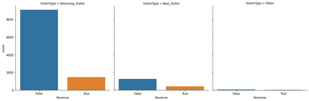
More revenue conversions happen for returning customers than new customers.

# Revenue Versus Traffic Type
sns.countplot(x="TrafficType", hue="Revenue", data=dataset)
plt.legend(loc="right")
plt.show()

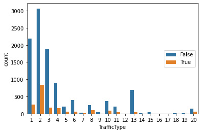
Most revenue conversion happens for web traffic generated from source 2.

Relationship between Revenue and Other Variables

sns.countplot(x="Region", hue="Revenue", data=dataset)
plt.show()

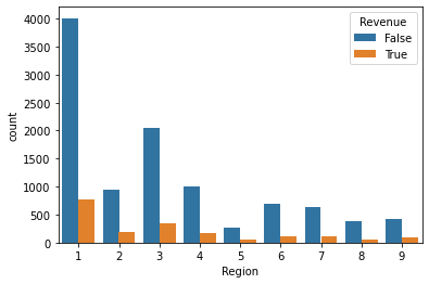
Region 1 accounts for most sales, and region 3 the second most.

sns.countplot(x="Browser", hue="Revenue", data=dataset)
plt.show()

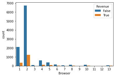
More revenue-generating transactions have been performed from Browser 2.

sns.countplot(x="OperatingSystems", hue="Revenue", data=dataset)
plt.show()

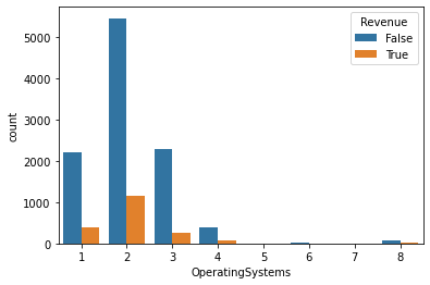
More revenue-generating transactions happened with OS 2 than the other types.

sns.countplot(
    x="Month",
    hue="Revenue",
    data=dataset,
    order=[
        "Feb",
        "Mar",
        "May",
        "June",
        "Jul",
        "Aug",
        "Sep",
        "Oct",
        "Nov",
        "Dec",
    ],
)
plt.show()

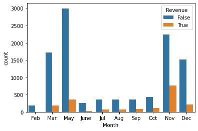
The greatest number of purchases were made in November.

Linear relationships

# Bounce Rate versus Exit Rate
sns.set(style="whitegrid")
ax = sns.lmplot(x="BounceRates", y="ExitRates", data=dataset)

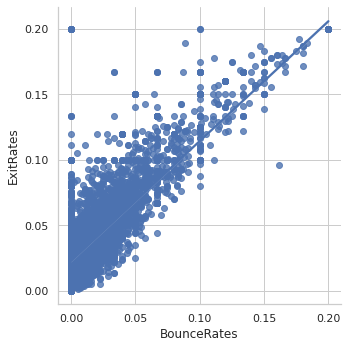
There is a positive correlation between the bounce rate and the exit rate. With the increase in bounce rate, the exit rate of the page increases.

# Page Value versus Bounce Rate
sns.set(style="whitegrid")
ax = sns.lmplot(x="PageValues", y="BounceRates", data=dataset)

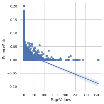
There is a negative correlation between page value and bounce rate. As the page value increases, the bounce rate decreases.

# Page Value versus Exit Rate
sns.set(style="whitegrid")
ax = sns.lmplot(x="PageValues", y="ExitRates", data=dataset)

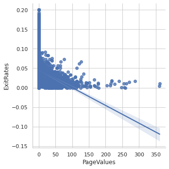
Negative correlation between page value and exit rate. Web pages with a better page value have a lower exit rate.

# Impact of Administration Page Views and
# Administrative Pageview Duration on Revenue
sns.set(style="whitegrid")
ax = sns.lmplot(
    x="Administrative",
    y="Administrative_Duration",
    hue="Revenue",
    data=dataset,
)

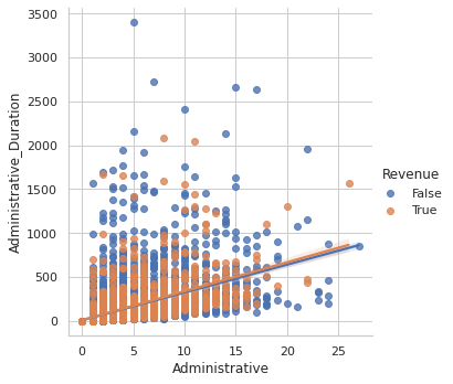
Administrative-related pageviews and the administrative-related pageview duration are positively correlated. When there is an increase in the number of administrative pageviews, the administrative pageview duration also increases.

# Impact of Information Page Views and Information Pageview Duration on Revenue
sns.set(style="whitegrid")
ax = sns.lmplot(
    x="Informational", y="Informational_Duration", hue="Revenue", data=dataset
)

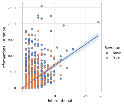
Information page views and information pageview duration are positively correlated. Customers who have made online purchases visited fewer numbers of informational pages. This implies that informational pageviews do not have much effect on revenue generation.