ARIMA models#
Autoregressive Integrated Moving Average (ARIMA) models are a class of statistical models that try to explain the behavior of a time series using its own past values. Being a class of models, ARIMA models are defined by a set of parameters (p,d,q), each one corresponding to a different component of the ARIMA model.
Importing libraries and packages#
 1# Warnings
 2import warnings
 3
 4# Mathematical operations and data manipulation
 5import pandas as pd
 6
 7# Models
 8from pmdarima import auto_arima
 9
10# Statistics
11from statsmodels.graphics.tsaplots import plot_acf, plot_pacf
12
13# Plotting
14import matplotlib.pyplot as plt
15
16warnings.filterwarnings("ignore")
17%matplotlib inline
---------------------------------------------------------------------------
ImportError                               Traceback (most recent call last)
Input In [1], in <cell line: 8>()
      5 import pandas as pd
      7 # Models
----> 8 from pmdarima import auto_arima
     10 # Statistics
     11 from statsmodels.graphics.tsaplots import plot_acf, plot_pacf

File ~/checkouts/readthedocs.org/user_builds/analysing/conda/latest/lib/python3.9/site-packages/pmdarima/__init__.py:52, in <module>
     49 from . import __check_build
     51 # Stuff we want at top-level
---> 52 from .arima import auto_arima, ARIMA, AutoARIMA, StepwiseContext, decompose
     53 from .utils import acf, autocorr_plot, c, pacf, plot_acf, plot_pacf, \
     54     tsdisplay
     55 from .utils._show_versions import show_versions

File ~/checkouts/readthedocs.org/user_builds/analysing/conda/latest/lib/python3.9/site-packages/pmdarima/arima/__init__.py:5, in <module>
      1 # -*- coding: utf-8 -*-
      2 #
      3 # Author: Taylor Smith <taylor.smith@alkaline-ml.com>
----> 5 from .approx import *
      6 from .arima import *
      7 from .auto import *

File ~/checkouts/readthedocs.org/user_builds/analysing/conda/latest/lib/python3.9/site-packages/pmdarima/arima/approx.py:9, in <module>
      1 # -*- coding: utf-8 -*-
      2 #
      3 # Author: Taylor Smith <taylor.smith@alkaline-ml.com>
      4 #
      5 # R approx function
      7 import numpy as np
----> 9 from ..utils.array import c, check_endog
     10 from ..utils import get_callable
     11 from ..compat.numpy import DTYPE

File ~/checkouts/readthedocs.org/user_builds/analysing/conda/latest/lib/python3.9/site-packages/pmdarima/utils/__init__.py:7, in <module>
      5 from .array import *
      6 from .metaestimators import *
----> 7 from .visualization import *
      8 from .wrapped import *
     11 def get_callable(key, dct):

File ~/checkouts/readthedocs.org/user_builds/analysing/conda/latest/lib/python3.9/site-packages/pmdarima/utils/visualization.py:11, in <module>
      8 from ..compat.pandas import plotting as pd_plotting
      9 from ..compat.matplotlib import get_compatible_pyplot
---> 11 from statsmodels.graphics import tsaplots
     13 import numpy as np
     14 import os

File ~/checkouts/readthedocs.org/user_builds/analysing/conda/latest/lib/python3.9/site-packages/statsmodels/graphics/tsaplots.py:11, in <module>
      8 import pandas as pd
     10 from statsmodels.graphics import utils
---> 11 from statsmodels.tsa.stattools import acf, pacf
     14 def _prepare_data_corr_plot(x, lags, zero):
     15     zero = bool(zero)

File ~/checkouts/readthedocs.org/user_builds/analysing/conda/latest/lib/python3.9/site-packages/statsmodels/tsa/stattools.py:19, in <module>
     17 from scipy import stats
     18 from scipy.interpolate import interp1d
---> 19 from scipy.signal import correlate
     21 from statsmodels.regression.linear_model import OLS, yule_walker
     22 from statsmodels.tools.sm_exceptions import (
     23     CollinearityWarning,
     24     InfeasibleTestError,
     25     InterpolationWarning,
     26     MissingDataError,
     27 )

File ~/checkouts/readthedocs.org/user_builds/analysing/conda/latest/lib/python3.9/site-packages/scipy/signal/__init__.py:309, in <module>
      1 """
      2 =======================================
      3 Signal processing (:mod:`scipy.signal`)
   (...)
    307
    308 """
--> 309 from . import _sigtools, windows
    310 from ._waveforms import *
    311 from ._max_len_seq import max_len_seq

File ~/checkouts/readthedocs.org/user_builds/analysing/conda/latest/lib/python3.9/site-packages/scipy/signal/windows/__init__.py:41, in <module>
      1 """
      2 Window functions (:mod:`scipy.signal.windows`)
      3 ==============================================
   (...)
     38
     39 """
---> 41 from ._windows import *
     43 # Deprecated namespaces, to be removed in v2.0.0
     44 from . import windows

File ~/checkouts/readthedocs.org/user_builds/analysing/conda/latest/lib/python3.9/site-packages/scipy/signal/windows/_windows.py:7, in <module>
      4 import warnings
      6 import numpy as np
----> 7 from scipy import linalg, special, fft as sp_fft
      9 __all__ = ['boxcar', 'triang', 'parzen', 'bohman', 'blackman', 'nuttall',
     10            'blackmanharris', 'flattop', 'bartlett', 'hanning', 'barthann',
     11            'hamming', 'kaiser', 'gaussian', 'general_cosine',
     12            'general_gaussian', 'general_hamming', 'chebwin', 'cosine',
     13            'hann', 'exponential', 'tukey', 'taylor', 'dpss', 'get_window']
     16 def _len_guards(M):

File ~/checkouts/readthedocs.org/user_builds/analysing/conda/latest/lib/python3.9/site-packages/scipy/fft/__init__.py:91, in <module>
     89 from ._realtransforms import dct, idct, dst, idst, dctn, idctn, dstn, idstn
     90 from ._fftlog import fht, ifht, fhtoffset
---> 91 from ._helper import next_fast_len
     92 from ._backend import (set_backend, skip_backend, set_global_backend,
     93                        register_backend)
     94 from numpy.fft import fftfreq, rfftfreq, fftshift, ifftshift

File ~/checkouts/readthedocs.org/user_builds/analysing/conda/latest/lib/python3.9/site-packages/scipy/fft/_helper.py:3, in <module>
      1 from functools import update_wrapper, lru_cache
----> 3 from ._pocketfft import helper as _helper
      6 def next_fast_len(target, real=False):
      7     """Find the next fast size of input data to ``fft``, for zero-padding, etc.
      8
      9     SciPy's FFT algorithms gain their speed by a recursive divide and conquer
   (...)
     59
     60     """

File ~/checkouts/readthedocs.org/user_builds/analysing/conda/latest/lib/python3.9/site-packages/scipy/fft/_pocketfft/__init__.py:3, in <module>
      1 """ FFT backend using pypocketfft """
----> 3 from .basic import *
      4 from .realtransforms import *
      5 from .helper import *

File ~/checkouts/readthedocs.org/user_builds/analysing/conda/latest/lib/python3.9/site-packages/scipy/fft/_pocketfft/basic.py:6, in <module>
      4 import numpy as np
      5 import functools
----> 6 from . import pypocketfft as pfft
      7 from .helper import (_asfarray, _init_nd_shape_and_axes, _datacopied,
      8                      _fix_shape, _fix_shape_1d, _normalization,
      9                      _workers)
     11 def c2c(forward, x, n=None, axis=-1, norm=None, overwrite_x=False,
     12         workers=None, *, plan=None):

ImportError: /home/docs/checkouts/readthedocs.org/user_builds/analysing/conda/latest/lib/python3.9/site-packages/zmq/backend/cython/../../../../.././libstdc++.so.6: version `GLIBCXX_3.4.30' not found (required by /home/docs/checkouts/readthedocs.org/user_builds/analysing/conda/latest/lib/python3.9/site-packages/scipy/fft/_pocketfft/pypocketfft.cpython-39-x86_64-linux-gnu.so)
Set paths#
1# Path to datasets directory
2data_path = "./datasets"
3# Path to assets directory (for saving results to)
4assets_path = "./assets"
Loading dataset#
1# load hourly data
2dataset = pd.read_csv(f"{data_path}/preprocessed_hour.csv")
3dataset.head()
| instant | dteday | season | yr | mnth | hr | holiday | weekday | workingday | weathersit | temp | atemp | hum | windspeed | casual | registered | cnt | |
|---|---|---|---|---|---|---|---|---|---|---|---|---|---|---|---|---|---|
| 0 | 1 | 2011-01-01 | winter | 2011 | 1 | 0 | 0 | Saturday | 0 | clear | 0.24 | 0.2879 | 81.0 | 0.0 | 3 | 13 | 16 |
| 1 | 2 | 2011-01-01 | winter | 2011 | 1 | 1 | 0 | Saturday | 0 | clear | 0.22 | 0.2727 | 80.0 | 0.0 | 8 | 32 | 40 |
| 2 | 3 | 2011-01-01 | winter | 2011 | 1 | 2 | 0 | Saturday | 0 | clear | 0.22 | 0.2727 | 80.0 | 0.0 | 5 | 27 | 32 |
| 3 | 4 | 2011-01-01 | winter | 2011 | 1 | 3 | 0 | Saturday | 0 | clear | 0.24 | 0.2879 | 75.0 | 0.0 | 3 | 10 | 13 |
| 4 | 5 | 2011-01-01 | winter | 2011 | 1 | 4 | 0 | Saturday | 0 | clear | 0.24 | 0.2879 | 75.0 | 0.0 | 0 | 1 | 1 |
1# print some generic statistics about the data
2print(f"Shape of data: {dataset.shape}")
3print(f"Number of missing values in the data: {dataset.isnull().sum().sum()}")
4
5# get statistics on the numerical columns
6dataset.describe().T
Shape of data: (17379, 17)
Number of missing values in the data: 0
| count | mean | std | min | 25% | 50% | 75% | max | |
|---|---|---|---|---|---|---|---|---|
| instant | 17379.0 | 8690.000000 | 5017.029500 | 1.00 | 4345.5000 | 8690.0000 | 13034.5000 | 17379.0000 |
| yr | 17379.0 | 2011.502561 | 0.500008 | 2011.00 | 2011.0000 | 2012.0000 | 2012.0000 | 2012.0000 |
| mnth | 17379.0 | 6.537775 | 3.438776 | 1.00 | 4.0000 | 7.0000 | 10.0000 | 12.0000 |
| hr | 17379.0 | 11.546752 | 6.914405 | 0.00 | 6.0000 | 12.0000 | 18.0000 | 23.0000 |
| holiday | 17379.0 | 0.028770 | 0.167165 | 0.00 | 0.0000 | 0.0000 | 0.0000 | 1.0000 |
| workingday | 17379.0 | 0.682721 | 0.465431 | 0.00 | 0.0000 | 1.0000 | 1.0000 | 1.0000 |
| temp | 17379.0 | 0.496987 | 0.192556 | 0.02 | 0.3400 | 0.5000 | 0.6600 | 1.0000 |
| atemp | 17379.0 | 0.475775 | 0.171850 | 0.00 | 0.3333 | 0.4848 | 0.6212 | 1.0000 |
| hum | 17379.0 | 62.722884 | 19.292983 | 0.00 | 48.0000 | 63.0000 | 78.0000 | 100.0000 |
| windspeed | 17379.0 | 12.736540 | 8.196795 | 0.00 | 7.0015 | 12.9980 | 16.9979 | 56.9969 |
| casual | 17379.0 | 35.676218 | 49.305030 | 0.00 | 4.0000 | 17.0000 | 48.0000 | 367.0000 |
| registered | 17379.0 | 153.786869 | 151.357286 | 0.00 | 34.0000 | 115.0000 | 220.0000 | 886.0000 |
| cnt | 17379.0 | 189.463088 | 181.387599 | 1.00 | 40.0000 | 142.0000 | 281.0000 | 977.0000 |
Preprocessing#
1# get daily rides
2daily_rides = dataset[["dteday", "registered", "casual"]]
3daily_rides = daily_rides.groupby("dteday").sum()
4
5# convert index to DateTime object
6daily_rides.index = pd.to_datetime(daily_rides.index)
 1# make time series stationary
 2registered = daily_rides["registered"]
 3registered_ma = registered.rolling(10).mean()
 4registered_ma_diff = registered - registered_ma
 5registered_ma_diff.dropna(inplace=True)
 6
 7casual = daily_rides["casual"]
 8casual_ma = casual.rolling(10).mean()
 9casual_ma_diff = casual - casual_ma
10casual_ma_diff.dropna(inplace=True)
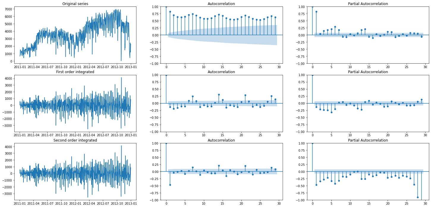
ACF and PACF plots for registered rides#
 1fig, axes = plt.subplots(3, 3, figsize=(25, 12))
 2
 3# Plotting original series
 4original = daily_rides["registered"]
 5axes[0, 0].plot(original)
 6axes[0, 0].set_title("Original series")
 7plot_acf(original, ax=axes[0, 1])
 8plot_pacf(original, ax=axes[0, 2])
 9
10# Plotting first order integrated series
11first_order_int = original.diff().dropna()
12axes[1, 0].plot(first_order_int)
13axes[1, 0].set_title("First order integrated")
14plot_acf(first_order_int, ax=axes[1, 1])
15plot_pacf(first_order_int, ax=axes[1, 2])
16
17# Plotting first order integrated series
18second_order_int = first_order_int.diff().dropna()
19axes[2, 0].plot(first_order_int)
20axes[2, 0].set_title("Second order integrated")
21plot_acf(second_order_int, ax=axes[2, 1])
22plot_pacf(second_order_int, ax=axes[2, 2])
23
24fig.savefig(f"{assets_path}/acf_pacf.png", format="png")
 1# Fitting an ARIMA model to the registered rides
 2model = auto_arima(
 3    registered,
 4    start_p=1,
 5    start_q=1,
 6    max_p=3,
 7    max_q=3,
 8    information_criterion="aic",
 9)
10
11print(model.summary())
                               SARIMAX Results
==============================================================================
Dep. Variable:                      y   No. Observations:                  731
Model:               SARIMAX(3, 1, 3)   Log Likelihood               -5854.491
Date:                Sun, 20 Mar 2022   AIC                          11722.982
Time:                        21:28:04   BIC                          11755.133
Sample:                             0   HQIC                         11735.386
                                - 731
Covariance Type:                  opg
==============================================================================
                 coef    std err          z      P>|z|      [0.025      0.975]
------------------------------------------------------------------------------
ar.L1          1.6077      0.050     32.421      0.000       1.511       1.705
ar.L2         -1.4474      0.062    -23.372      0.000      -1.569      -1.326
ar.L3          0.3608      0.049      7.396      0.000       0.265       0.456
ma.L1         -2.1153      0.034    -62.375      0.000      -2.182      -2.049
ma.L2          2.0601      0.047     43.824      0.000       1.968       2.152
ma.L3         -0.8605      0.032    -27.085      0.000      -0.923      -0.798
sigma2      6.239e+05   2.42e+04     25.784      0.000    5.77e+05    6.71e+05
===================================================================================
Ljung-Box (L1) (Q):                   0.38   Jarque-Bera (JB):               756.72
Prob(Q):                              0.54   Prob(JB):                         0.00
Heteroskedasticity (H):               3.35   Skew:                            -1.32
Prob(H) (two-sided):                  0.00   Kurtosis:                         7.23
===================================================================================

Warnings:
[1] Covariance matrix calculated using the outer product of gradients (complex-step).
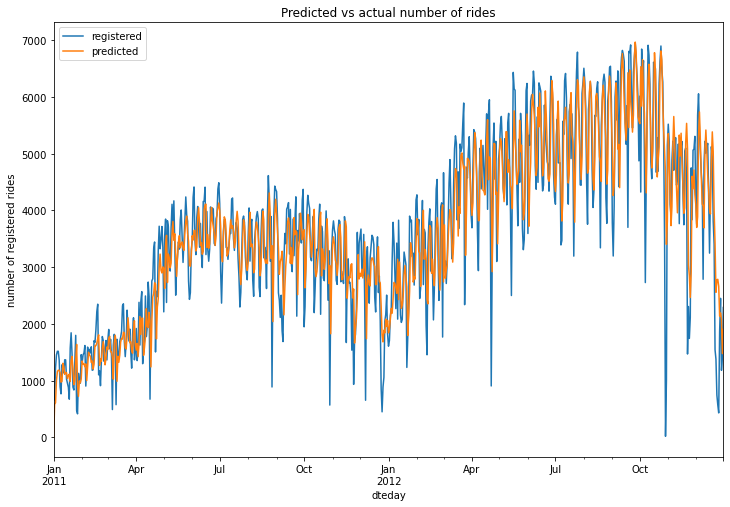
1# plot original and predicted values
2plot_data = pd.DataFrame(registered)
3plot_data["predicted"] = model.predict_in_sample()
4plot_data.plot(figsize=(12, 8))
5plt.ylabel("number of registered rides")
6plt.title("Predicted vs actual number of rides")
7plt.savefig(f"{assets_path}/registered_arima_fit.png", format="png")