Preprocessing

Loading the data and performing some initial exploration on it to acquire some basic knowledge about the data, how the various features are distributed.

Importing libraries and packages

# Mathematical operations and data manipulation
import pandas as pd

# Plotting
import seaborn as sns

# Warnings
import warnings

warnings.filterwarnings("ignore")
%matplotlib inline

Set paths

# Path to datasets directory
data_path = "./datasets"
# Path to assets directory (for saving results to)
assets_path = "./assets"

Loading dataset

# load data
dataset = pd.read_csv(f"{data_path}/preprocessed_energydata.csv")
dataset.head().T

	0	1	2	3	4
date_time	2016-01-11 17:00:00	2016-01-11 17:10:00	2016-01-11 17:20:00	2016-01-11 17:30:00	2016-01-11 17:40:00
a_energy	60	60	50	50	60
l_energy	30	30	30	40	40
kitchen_temp	19.89	19.89	19.89	19.89	19.89
kitchen_hum	47.596667	46.693333	46.3	46.066667	46.333333
liv_temp	19.2	19.2	19.2	19.2	19.2
liv_hum	44.79	44.7225	44.626667	44.59	44.53
laun_temp	19.79	19.79	19.79	19.79	19.79
laun_hum	44.73	44.79	44.933333	45.0	45.0
off_temp	19.0	19.0	18.926667	18.89	18.89
off_hum	45.566667	45.9925	45.89	45.723333	45.53
bath_temp	17.166667	17.166667	17.166667	17.166667	17.2
bath_hum	55.2	55.2	55.09	55.09	55.09
out_b_temp	7.026667	6.833333	6.56	6.433333	6.366667
out_b_hum	84.256667	84.063333	83.156667	83.423333	84.893333
iron_temp	17.2	17.2	17.2	17.133333	17.2
iron_hum	41.626667	41.56	41.433333	41.29	41.23
teen_temp	18.2	18.2	18.2	18.1	18.1
teen_hum	48.9	48.863333	48.73	48.59	48.59
par_temp	17.033333	17.066667	17.0	17.0	17.0
par_hum	45.53	45.56	45.5	45.4	45.4
out_temp	6.6	6.483333	6.366667	6.25	6.133333
out_press	733.5	733.6	733.7	733.8	733.9
out_hum	92.0	92.0	92.0	92.0	92.0
wind	7.0	6.666667	6.333333	6.0	5.666667
visibility	63.0	59.166667	55.333333	51.5	47.666667
dew_point	5.3	5.2	5.1	5.0	4.9
rv1	13.275433	18.606195	28.642668	45.410389	10.084097
rv2	13.275433	18.606195	28.642668	45.410389	10.084097

Outliers and missing values

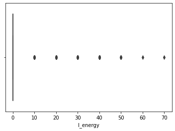
Analysing the Light Energy Consumption Column

lights_box = sns.boxplot(dataset.l_energy)

lst = [0, 10, 20, 30, 40, 50, 60, 70]
counts = []

for i in lst:
    a = (dataset.l_energy == i).sum()
    counts.append(a)

print(counts)

[15252, 2212, 1624, 559, 77, 9, 1, 1]

lights = sns.barplot(x=lst, y=counts)
lights.set_xlabel("Energy Consumed by Lights")
lights.set_ylabel("Number of Lights")
lights.set_title("Distribution of Energy Consumed by Lights")

Text(0.5, 1.0, 'Distribution of Energy Consumed by Lights')

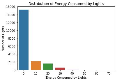
((dataset.l_energy == 0).sum() / (dataset.shape[0])) * 100

77.28401317456296

77% of the instances have 0 Wh. This renders the l_energy column useless because we can’t possibly find any links between it and the other data.

new_data = dataset
new_data.drop(["l_energy"], axis=1, inplace=True)

new_data.head().T

	0	1	2	3	4
date_time	2016-01-11 17:00:00	2016-01-11 17:10:00	2016-01-11 17:20:00	2016-01-11 17:30:00	2016-01-11 17:40:00
a_energy	60	60	50	50	60
kitchen_temp	19.89	19.89	19.89	19.89	19.89
kitchen_hum	47.596667	46.693333	46.3	46.066667	46.333333
liv_temp	19.2	19.2	19.2	19.2	19.2
liv_hum	44.79	44.7225	44.626667	44.59	44.53
laun_temp	19.79	19.79	19.79	19.79	19.79
laun_hum	44.73	44.79	44.933333	45.0	45.0
off_temp	19.0	19.0	18.926667	18.89	18.89
off_hum	45.566667	45.9925	45.89	45.723333	45.53
bath_temp	17.166667	17.166667	17.166667	17.166667	17.2
bath_hum	55.2	55.2	55.09	55.09	55.09
out_b_temp	7.026667	6.833333	6.56	6.433333	6.366667
out_b_hum	84.256667	84.063333	83.156667	83.423333	84.893333
iron_temp	17.2	17.2	17.2	17.133333	17.2
iron_hum	41.626667	41.56	41.433333	41.29	41.23
teen_temp	18.2	18.2	18.2	18.1	18.1
teen_hum	48.9	48.863333	48.73	48.59	48.59
par_temp	17.033333	17.066667	17.0	17.0	17.0
par_hum	45.53	45.56	45.5	45.4	45.4
out_temp	6.6	6.483333	6.366667	6.25	6.133333
out_press	733.5	733.6	733.7	733.8	733.9
out_hum	92.0	92.0	92.0	92.0	92.0
wind	7.0	6.666667	6.333333	6.0	5.666667
visibility	63.0	59.166667	55.333333	51.5	47.666667
dew_point	5.3	5.2	5.1	5.0	4.9
rv1	13.275433	18.606195	28.642668	45.410389	10.084097
rv2	13.275433	18.606195	28.642668	45.410389	10.084097

Analysing the Appliances Energy Consumption Column

app_box = sns.boxplot(new_data.a_energy)

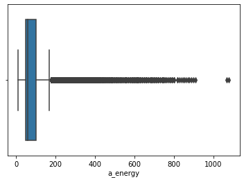
A majority of the values seem to lie between 50 Wh and 100 Wh. However, some values extend the upper bracket of 200 Wh and go beyond 1000 Wh.

# Check to see how many values extend above 200 Wh.
out = (new_data["a_energy"] > 200).sum()
out

1916

# The percentage of the number of instances wherein the value
# of the energy consumed by appliances is above 200 Wh
(out / 19735) * 100

9.708639473017481

# The total number of instances wherein the value of the energy
# consumed by appliances is above 950 Wh.
out_e = (new_data["a_energy"] > 950).sum()
out_e

2

# The percentage of the number of instances wherein the value of
# the energy consumed by appliances is above 950 Wh.
(out_e / 19735) * 100

0.010134279199391943

Only 0.01% of the instances have a_energy above 950 Wh. Close to 10% of the instances have a_energy above 200 Wh. Deleting (for now).

energy = new_data[(new_data["a_energy"] <= 200)]
energy.describe()

	a_energy	kitchen_temp	kitchen_hum	liv_temp	liv_hum	laun_temp	laun_hum	off_temp	off_hum	bath_temp	...	par_temp	par_hum	out_temp	out_press	out_hum	wind	visibility	dew_point	rv1	rv2
count	17819.000000	17819.000000	17819.000000	17819.000000	17819.000000	17819.000000	17819.000000	17819.000000	17819.000000	17819.000000	...	17819.000000	17819.000000	17819.000000	17819.000000	17819.000000	17819.000000	17819.000000	17819.000000	17819.000000	17819.000000
mean	68.728324	21.687676	40.158323	20.294921	40.470961	22.230049	39.167393	20.858577	38.991000	19.607705	...	19.502262	41.556127	7.315671	755.559383	80.236718	3.975014	38.306600	3.762120	25.002765	25.002765
std	31.378141	1.605252	3.933742	2.172435	4.062130	1.971209	3.223465	2.048053	4.324842	1.838655	...	2.011673	4.164766	5.290522	7.345043	14.771215	2.448213	11.951954	4.186178	14.519549	14.519549
min	10.000000	16.790000	27.023333	16.100000	20.463333	17.200000	28.766667	15.100000	27.660000	15.330000	...	14.890000	29.166667	-5.000000	729.366667	24.000000	0.000000	1.000000	-6.600000	0.005322	0.005322
25%	50.000000	20.760000	37.260000	18.790000	37.930000	20.790000	36.826667	19.566667	35.500000	18.290000	...	18.066667	38.530000	3.533333	751.000000	71.166667	2.000000	29.000000	0.933333	12.461009	12.461009
50%	60.000000	21.600000	39.560000	19.926667	40.560000	22.100000	38.471429	20.666667	38.363333	19.390000	...	19.390000	40.863333	6.850000	756.100000	84.333333	3.500000	40.000000	3.433333	24.940753	24.940753
75%	80.000000	22.600000	42.900000	21.472333	43.326667	23.290000	41.590000	22.100000	42.090000	20.600000	...	20.600000	44.296667	10.333333	760.933333	91.845238	5.333333	40.000000	6.550000	37.660263	37.660263
max	200.000000	26.200000	59.633333	29.856667	56.026667	29.200000	49.656667	26.200000	51.000000	25.795000	...	24.500000	53.326667	26.100000	772.283333	100.000000	14.000000	66.000000	15.500000	49.996530	49.996530

8 rows × 27 columns

energy.to_csv(f"{data_path}/cleaned_energydata.csv", index=False)