Preprocessing

Loading the data and performing some initial exploration on it to acquire some basic knowledge about the data, how the various features are distributed.

Importing libraries and packages

# Mathematical operations and data manipulation
import pandas as pd

# Plotting
import seaborn as sns
import matplotlib.pyplot as plt

# Warnings
import warnings

warnings.filterwarnings("ignore")

%matplotlib inline

Set paths

# Path to datasets directory
data_path = "./datasets"
# Path to assets directory (for saving results to)
assets_path = "./assets"

Loading dataset

# load data
dataset = pd.read_csv(f"{data_path}/hour.csv")
dataset.head()

	instant	dteday	season	yr	mnth	hr	holiday	weekday	workingday	weathersit	temp	atemp	hum	windspeed	casual	registered	cnt
0	1	2011-01-01	1	0	1	0	0	6	0	1	0.24	0.2879	0.81	0.0	3	13	16
1	2	2011-01-01	1	0	1	1	0	6	0	1	0.22	0.2727	0.80	0.0	8	32	40
2	3	2011-01-01	1	0	1	2	0	6	0	1	0.22	0.2727	0.80	0.0	5	27	32
3	4	2011-01-01	1	0	1	3	0	6	0	1	0.24	0.2879	0.75	0.0	3	10	13
4	5	2011-01-01	1	0	1	4	0	6	0	1	0.24	0.2879	0.75	0.0	0	1	1

Exploring dataset

# Shape and missing data
print(f"Shape of data: {dataset.shape}")
print(f"Number of missing values in the data: {dataset.isnull().sum().sum()}")

# Statistics on the numerical columns
dataset.describe().T

Shape of data: (17379, 17)
Number of missing values in the data: 0

	count	mean	std	min	25%	50%	75%	max
instant	17379.0	8690.000000	5017.029500	1.00	4345.5000	8690.0000	13034.5000	17379.0000
season	17379.0	2.501640	1.106918	1.00	2.0000	3.0000	3.0000	4.0000
yr	17379.0	0.502561	0.500008	0.00	0.0000	1.0000	1.0000	1.0000
mnth	17379.0	6.537775	3.438776	1.00	4.0000	7.0000	10.0000	12.0000
hr	17379.0	11.546752	6.914405	0.00	6.0000	12.0000	18.0000	23.0000
holiday	17379.0	0.028770	0.167165	0.00	0.0000	0.0000	0.0000	1.0000
weekday	17379.0	3.003683	2.005771	0.00	1.0000	3.0000	5.0000	6.0000
workingday	17379.0	0.682721	0.465431	0.00	0.0000	1.0000	1.0000	1.0000
weathersit	17379.0	1.425283	0.639357	1.00	1.0000	1.0000	2.0000	4.0000
temp	17379.0	0.496987	0.192556	0.02	0.3400	0.5000	0.6600	1.0000
atemp	17379.0	0.475775	0.171850	0.00	0.3333	0.4848	0.6212	1.0000
hum	17379.0	0.627229	0.192930	0.00	0.4800	0.6300	0.7800	1.0000
windspeed	17379.0	0.190098	0.122340	0.00	0.1045	0.1940	0.2537	0.8507
casual	17379.0	35.676218	49.305030	0.00	4.0000	17.0000	48.0000	367.0000
registered	17379.0	153.786869	151.357286	0.00	34.0000	115.0000	220.0000	886.0000
cnt	17379.0	189.463088	181.387599	1.00	40.0000	142.0000	281.0000	977.0000

Preprocessing temporal and weather features

def transform_seasons(data):
    # Tranforming seasons
    seasons_mapping = {1: "winter", 2: "spring", 3: "summer", 4: "fall"}
    data["season"] = data["season"].apply(lambda x: seasons_mapping[x])
    return data


def transform_yr(data):
    # Transforming yr
    yr_mapping = {0: 2011, 1: 2012}
    data["yr"] = data["yr"].apply(lambda x: yr_mapping[x])
    return data


def transform_weekday(data):
    # Transforming weekday
    weekday_mapping = {
        0: "Sunday",
        1: "Monday",
        2: "Tuesday",
        3: "Wednesday",
        4: "Thursday",
        5: "Friday",
        6: "Saturday",
    }
    data["weekday"] = data["weekday"].apply(lambda x: weekday_mapping[x])
    return data


def transform_weathersit(data):
    # Transforming weathersit
    weather_mapping = {
        1: "clear",
        2: "cloudy",
        3: "light_rain_snow",
        4: "heavy_rain_snow",
    }
    data["weathersit"] = data["weathersit"].apply(lambda x: weather_mapping[x])
    return data


def transform_hum(data):
    # Transorming humidity
    data["hum"] = data["hum"] * 100
    return data


def transform_windspeed(data):
    # Transorming windspeed
    data["windspeed"] = data["windspeed"] * 67
    return data


def preprocess(data):
    data = transform_seasons(data)
    data = transform_yr(data)
    data = transform_weekday(data)
    data = transform_weathersit(data)
    data = transform_hum(data)
    data = transform_windspeed(data)
    return data


preprocessed_data = preprocess(dataset)
preprocessed_data.to_csv(f"{data_path}/preprocessed_hour.csv", index=False)

# Visualizing preprocessed columns
cols = ["season", "yr", "weekday", "weathersit", "hum", "windspeed"]
preprocessed_data[cols].sample(10, random_state=42)

	season	yr	weekday	weathersit	hum	windspeed
12830	summer	2012	Saturday	clear	27.0	12.9980
8688	winter	2012	Monday	clear	41.0	15.0013
7091	fall	2011	Friday	clear	66.0	19.0012
12230	spring	2012	Tuesday	clear	52.0	23.9994
431	winter	2011	Thursday	clear	56.0	26.0027
1086	winter	2011	Friday	clear	72.0	19.0012
11605	spring	2012	Thursday	clear	58.0	8.9981
7983	fall	2011	Sunday	clear	87.0	0.0000
10391	winter	2012	Wednesday	clear	68.0	12.9980
7046	fall	2011	Wednesday	clear	71.0	15.0013

Registered vs casual use analysis

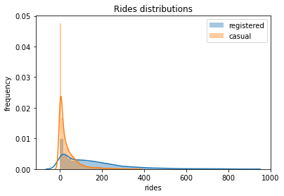
# Plotting distributions of registered vs casual rides
sns.distplot(preprocessed_data["registered"], label="registered")
sns.distplot(preprocessed_data["casual"], label="casual")
plt.legend()
plt.xlabel("rides")
plt.ylabel("frequency")
plt.title("Rides distributions")
plt.savefig(f"{assets_path}/rides_distributions.png", format="png")

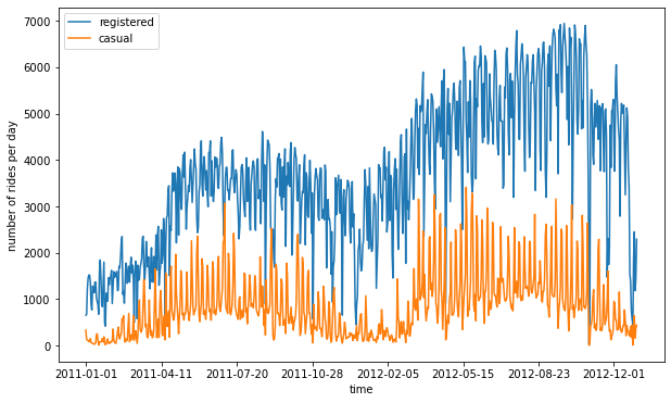
# Plotting rides over time
plot_data = preprocessed_data[["registered", "casual", "dteday"]]
ax = plot_data.groupby("dteday").sum().plot(figsize=(10, 6))
ax.set_xlabel("time")
ax.set_ylabel("number of rides per day")

plt.savefig(f"{assets_path}/rides_daily.png", format="png")

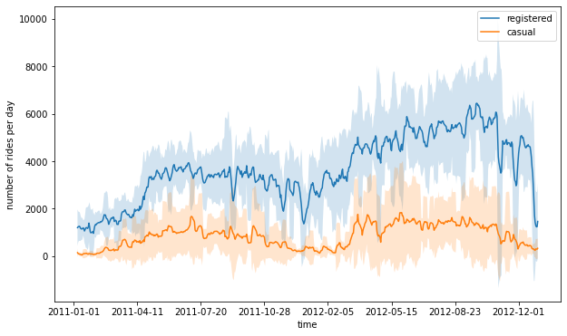
# Creating a new dataframe for plotting columns, and obtaining number
# of rides per day, by grouping over each day
plot_data = preprocessed_data[["registered", "casual", "dteday"]]
plot_data = plot_data.groupby("dteday").sum()

# Defining window for computing the rolling mean and standard deviation
window = 7
rolling_means = plot_data.rolling(window).mean()
rolling_deviations = plot_data.rolling(window).std()

# Creating a plot of the series, where we first plot the series of
# rolling means, then colouring the zone between the series of
# rolling means +- 2 rolling standard deviations
ax = rolling_means.plot(figsize=(10, 6))
ax.fill_between(
    rolling_means.index,
    rolling_means["registered"] + 2 * rolling_deviations["registered"],
    rolling_means["registered"] - 2 * rolling_deviations["registered"],
    alpha=0.2,
)
ax.fill_between(
    rolling_means.index,
    rolling_means["casual"] + 2 * rolling_deviations["casual"],
    rolling_means["casual"] - 2 * rolling_deviations["casual"],
    alpha=0.2,
)
ax.set_xlabel("time")
ax.set_ylabel("number of rides per day")
plt.savefig(f"{assets_path}/rides_aggregated.png", format="png")

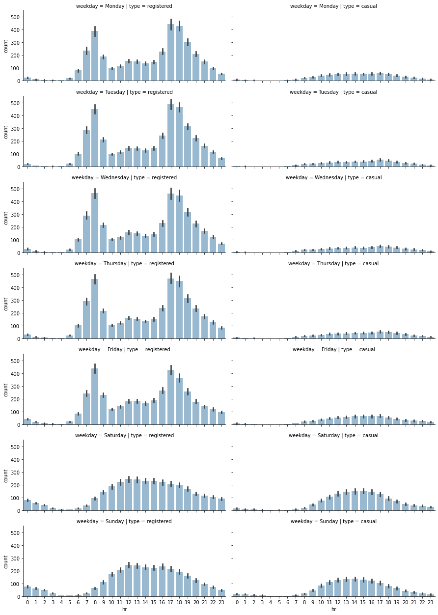
# Selecting relevant columns
plot_data = preprocessed_data[["hr", "weekday", "registered", "casual"]]

# Transforming the data into a format, in number of entries are computed
# as count, for each distinct hr, weekday and type (registered or casual)
plot_data = plot_data.melt(
    id_vars=["hr", "weekday"], var_name="type", value_name="count"
)

# Creating a FacetGrid object, in which a grid plot is produced.
# As columns, we have the various days of the week, as rows, the different
# types (registered and casual)
grid = sns.FacetGrid(
    plot_data,
    row="weekday",
    col="type",
    height=2.5,
    aspect=2.5,
    row_order=[
        "Monday",
        "Tuesday",
        "Wednesday",
        "Thursday",
        "Friday",
        "Saturday",
        "Sunday",
    ],
)

# Populating the FacetGrid with the specific plots
grid.map(sns.barplot, "hr", "count", alpha=0.5)
grid.savefig(f"{assets_path}/weekday_hour_distributions.png", format="png")

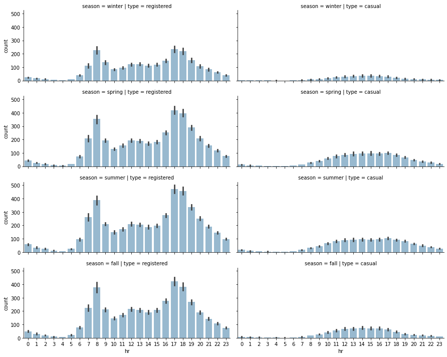
Analysing seasonal impact on rides

# Selecting subset of the data
plot_data = preprocessed_data[["hr", "season", "registered", "casual"]]

# Unpivoting data from wide to long format
plot_data = plot_data.melt(
    id_vars=["hr", "season"], var_name="type", value_name="count"
)

# Defining FacetGrid
grid = sns.FacetGrid(
    plot_data,
    row="season",
    col="type",
    height=2.5,
    aspect=2.5,
    row_order=["winter", "spring", "summer", "fall"],
)

# Applying plotting function to each element in the grid
grid.map(sns.barplot, "hr", "count", alpha=0.5)

# Saving figure
grid.savefig(f"{assets_path}/season_impact_a.png", format="png")

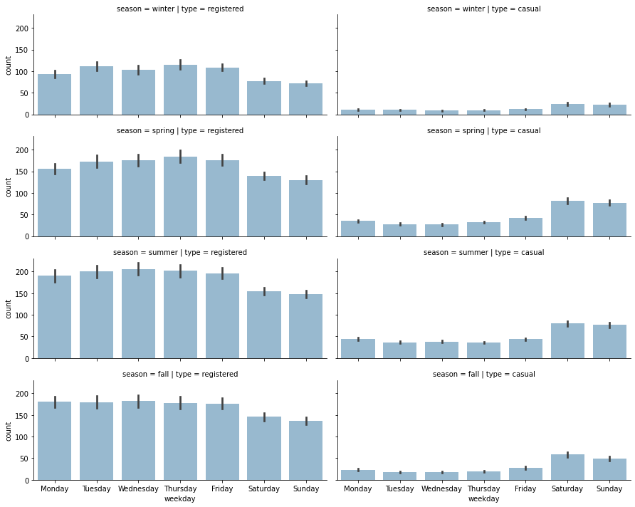
plot_data = preprocessed_data[["weekday", "season", "registered", "casual"]]
plot_data = plot_data.melt(
    id_vars=["weekday", "season"], var_name="type", value_name="count"
)

grid = sns.FacetGrid(
    plot_data,
    row="season",
    col="type",
    height=2.5,
    aspect=2.5,
    row_order=["winter", "spring", "summer", "fall"],
)
grid.map(
    sns.barplot,
    "weekday",
    "count",
    alpha=0.5,
    order=[
        "Monday",
        "Tuesday",
        "Wednesday",
        "Thursday",
        "Friday",
        "Saturday",
        "Sunday",
    ],
)

# Saving figure
grid.savefig(f"{assets_path}/season_impact_b.png", format="png")