Preprocessing#
Employees with higher education degrees, in positions of higher responsibility, might be less prone to being absent.
Importing libraries and packages#
 1# Mathematical operations and data manipulation
 2import pandas as pd
 3
 4# Plotting
 5import seaborn as sns
 6import matplotlib.pyplot as plt
 7
 8# Warnings
 9import warnings
10
11warnings.filterwarnings("ignore")
12
13%matplotlib inline
Set paths#
1# Path to datasets directory
2data_path = "./datasets"
3# Path to assets directory (for saving results to)
4assets_path = "./assets"
Loading dataset#
1# load data
2dataset = pd.read_csv(f"{data_path}/preprocessed_absenteism.csv")
3dataset.head()
| ID | Reason for absence | Month of absence | Day of the week | Seasons | Transportation expense | Distance from Residence to Work | Service time | Age | Work load Average/day | ... | Disciplinary failure | Education | Son | Social drinker | Social smoker | Pet | Weight | Height | Body mass index | Absenteeism time in hours | |
|---|---|---|---|---|---|---|---|---|---|---|---|---|---|---|---|---|---|---|---|---|---|
| 0 | 11 | 26 | July | Tuesday | Spring | 289 | 36 | 13 | 33 | 239.554 | ... | No | high_school | 2 | Yes | No | 1 | 90 | 172 | 30 | 4 |
| 1 | 36 | 0 | July | Tuesday | Spring | 118 | 13 | 18 | 50 | 239.554 | ... | Yes | high_school | 1 | Yes | No | 0 | 98 | 178 | 31 | 0 |
| 2 | 3 | 23 | July | Wednesday | Spring | 179 | 51 | 18 | 38 | 239.554 | ... | No | high_school | 0 | Yes | No | 0 | 89 | 170 | 31 | 2 |
| 3 | 7 | 7 | July | Thursday | Spring | 279 | 5 | 14 | 39 | 239.554 | ... | No | high_school | 2 | Yes | Yes | 0 | 68 | 168 | 24 | 4 |
| 4 | 11 | 23 | July | Thursday | Spring | 289 | 36 | 13 | 33 | 239.554 | ... | No | high_school | 2 | Yes | No | 1 | 90 | 172 | 30 | 2 |
5 rows × 21 columns
Exploring dataset#
1# Printing dimensionality of the data, columns, types and missing values
2print(f"Data dimension: {dataset.shape}")
3for col in dataset.columns:
4    print(
5        f"Column: {col:35} | "
6        f"type: {str(dataset[col].dtype):7} | "
7        f"missing values: {dataset[col].isna().sum():3d}"
8    )
Data dimension: (740, 21)
Column: ID                                  | type: int64   | missing values:   0
Column: Reason for absence                  | type: int64   | missing values:   0
Column: Month of absence                    | type: object  | missing values:   0
Column: Day of the week                     | type: object  | missing values:   0
Column: Seasons                             | type: object  | missing values:   0
Column: Transportation expense              | type: int64   | missing values:   0
Column: Distance from Residence to Work     | type: int64   | missing values:   0
Column: Service time                        | type: int64   | missing values:   0
Column: Age                                 | type: int64   | missing values:   0
Column: Work load Average/day               | type: float64 | missing values:   0
Column: Hit target                          | type: int64   | missing values:   0
Column: Disciplinary failure                | type: object  | missing values:   0
Column: Education                           | type: object  | missing values:   0
Column: Son                                 | type: int64   | missing values:   0
Column: Social drinker                      | type: object  | missing values:   0
Column: Social smoker                       | type: object  | missing values:   0
Column: Pet                                 | type: int64   | missing values:   0
Column: Weight                              | type: int64   | missing values:   0
Column: Height                              | type: int64   | missing values:   0
Column: Body mass index                     | type: int64   | missing values:   0
Column: Absenteeism time in hours           | type: int64   | missing values:   0
1# Computing statistics on numerical features
2dataset.describe().T
| count | mean | std | min | 25% | 50% | 75% | max | |
|---|---|---|---|---|---|---|---|---|
| ID | 740.0 | 18.017568 | 11.021247 | 1.000 | 9.000 | 18.000 | 28.000 | 36.000 |
| Reason for absence | 740.0 | 19.216216 | 8.433406 | 0.000 | 13.000 | 23.000 | 26.000 | 28.000 |
| Transportation expense | 740.0 | 221.329730 | 66.952223 | 118.000 | 179.000 | 225.000 | 260.000 | 388.000 |
| Distance from Residence to Work | 740.0 | 29.631081 | 14.836788 | 5.000 | 16.000 | 26.000 | 50.000 | 52.000 |
| Service time | 740.0 | 12.554054 | 4.384873 | 1.000 | 9.000 | 13.000 | 16.000 | 29.000 |
| Age | 740.0 | 36.450000 | 6.478772 | 27.000 | 31.000 | 37.000 | 40.000 | 58.000 |
| Work load Average/day | 740.0 | 271.490235 | 39.058116 | 205.917 | 244.387 | 264.249 | 294.217 | 378.884 |
| Hit target | 740.0 | 94.587838 | 3.779313 | 81.000 | 93.000 | 95.000 | 97.000 | 100.000 |
| Son | 740.0 | 1.018919 | 1.098489 | 0.000 | 0.000 | 1.000 | 2.000 | 4.000 |
| Pet | 740.0 | 0.745946 | 1.318258 | 0.000 | 0.000 | 0.000 | 1.000 | 8.000 |
| Weight | 740.0 | 79.035135 | 12.883211 | 56.000 | 69.000 | 83.000 | 89.000 | 108.000 |
| Height | 740.0 | 172.114865 | 6.034995 | 163.000 | 169.000 | 170.000 | 172.000 | 196.000 |
| Body mass index | 740.0 | 26.677027 | 4.285452 | 19.000 | 24.000 | 25.000 | 31.000 | 38.000 |
| Absenteeism time in hours | 740.0 | 6.924324 | 13.330998 | 0.000 | 2.000 | 3.000 | 8.000 | 120.000 |
Individual identification (ID)
Reason for absence (ICD). Absences attested by the International Code of Diseases (ICD) stratified into 21 categories (I to XXI) as follows:
I Certain infectious and parasitic diseases II Neoplasms III Diseases of the blood and blood-forming organs and certain disorders involving the immune mechanism IV Endocrine, nutritional and metabolic diseases V Mental and behavioural disorders VI Diseases of the nervous system VII Diseases of the eye and adnexa VIII Diseases of the ear and mastoid process IX Diseases of the circulatory system X Diseases of the respiratory system XI Diseases of the digestive system XII Diseases of the skin and subcutaneous tissue XIII Diseases of the musculoskeletal system and connective tissue XIV Diseases of the genitourinary system XV Pregnancy, childbirth and the puerperium XVI Certain conditions originating in the perinatal period XVII Congenital malformations, deformations and chromosomal abnormalities XVIII Symptoms, signs and abnormal clinical and laboratory findings, not elsewhere classified XIX Injury, poisoning and certain other consequences of external causes XX External causes of morbidity and mortality XXI Factors influencing health status and contact with health services.
And 7 categories without (CID) 2. patient follow-up (22), 3. medical consultation (23), 4. blood donation (24), 5. laboratory examination (25), 6. unjustified absence (26), 7. physiotherapy (27), 8. dental consultation (28).
Month of absence
Day of the week (Monday (2), Tuesday (3), Wednesday (4), Thursday (5), Friday (6))
Seasons (summer (1), autumn (2), winter (3), spring (4))
Transportation expense
Distance from Residence to Work (kilometers)
Service time
Age
Work load Average/day
Hit target
Disciplinary failure (yes=1; no=0)
Education (high school (1), graduate (2), postgraduate (3), master and doctor (4))
Son (number of children)
Social drinker (yes=1; no=0)
Social smoker (yes=1; no=0)
Pet (number of pet)
Weight
Height
Body mass index
Absenteeism time in hours (target)
Preprocessing#
1# Function to check if the provided integer value is contained
2# in the ICD or not
3def in_icd(val):
4    r = range(1, 22)
5    return "Yes" if val in r else "No"
6
7
8# Adding Disease column
9dataset["Disease"] = dataset["Reason for absence"].apply(in_icd)
Education plots#
 1# Computing percentage of employees per education level
 2education_types = ["high_school", "graduate", "postgraduate", "master_phd"]
 3counts = dataset["Education"].value_counts()
 4percentages = dataset["Education"].value_counts(normalize=True)
 5for educ_type in education_types:
 6    print(
 7        f"Education type: {educ_type:12s} | "
 8        f"Counts : {counts[educ_type]:6.0f} | "
 9        f"Percentage: {100*percentages[educ_type]:4.1f}"
10    )
Education type: high_school  | Counts :    611 | Percentage: 82.6
Education type: graduate     | Counts :     46 | Percentage:  6.2
Education type: postgraduate | Counts :     79 | Percentage: 10.7
Education type: master_phd   | Counts :      4 | Percentage:  0.5
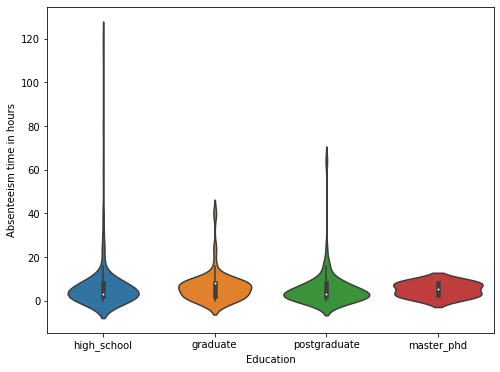
1# Distribution of absence hours, based on education level
2plt.figure(figsize=(8, 6))
3sns.violinplot(
4    x="Education",
5    y="Absenteeism time in hours",
6    data=dataset,
7    order=["high_school", "graduate", "postgraduate", "master_phd"],
8)
9plt.savefig(f"{assets_path}/violin_education_hours.png", format="png")
 1# Computing mean and standard deviation of absence hours
 2education_types = ["high_school", "graduate", "postgraduate", "master_phd"]
 3for educ_type in education_types:
 4    mask = dataset["Education"] == educ_type
 5    hours = dataset["Absenteeism time in hours"][mask]
 6    mean = hours.mean()
 7    stddev = hours.std()
 8    print(
 9        f"Education type: {educ_type:12s} | "
10        f"Mean : {mean:.03f} | "
11        f"Stddev: {stddev:.03f}"
12    )
Education type: high_school  | Mean : 7.190 | Stddev: 14.259
Education type: graduate     | Mean : 6.391 | Stddev: 6.754
Education type: postgraduate | Mean : 5.266 | Stddev: 7.963
Education type: master_phd   | Mean : 5.250 | Stddev: 3.202
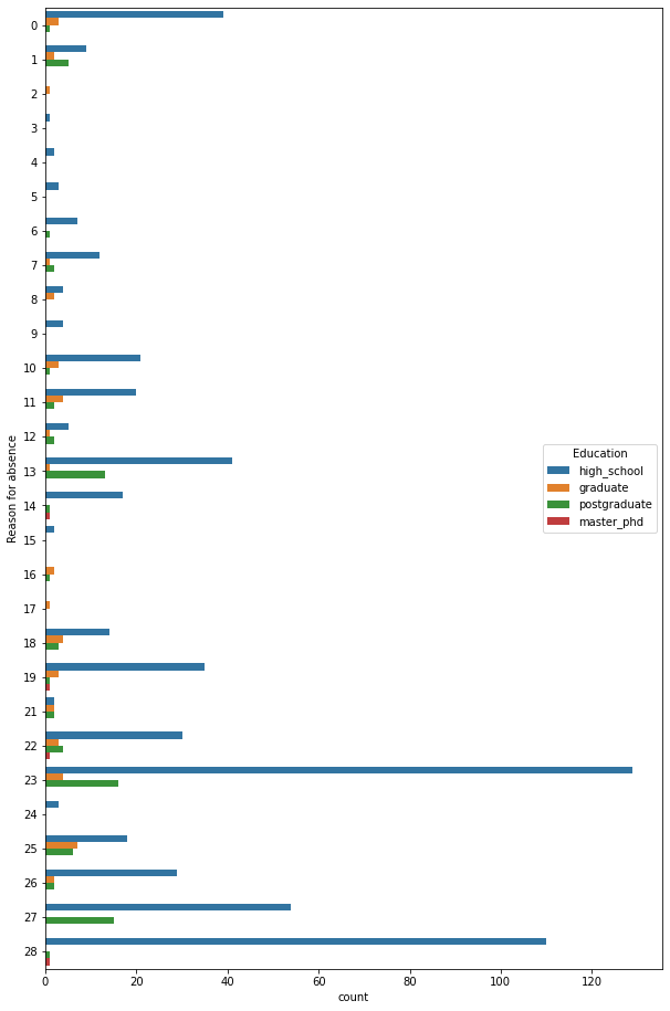
1# Plotting reason for absence, based on education level
2plt.figure(figsize=(10, 16))
3sns.countplot(
4    data=dataset,
5    y="Reason for absence",
6    hue="Education",
7    hue_order=["high_school", "graduate", "postgraduate", "master_phd"],
8)
9plt.savefig(f"{assets_path}/count_education_reason.png", format="png")