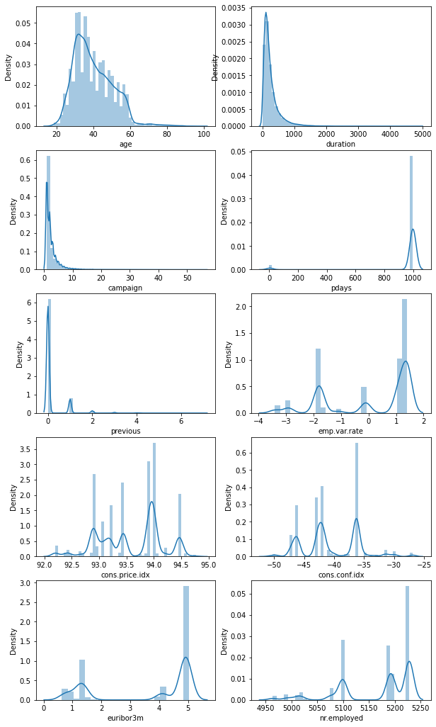
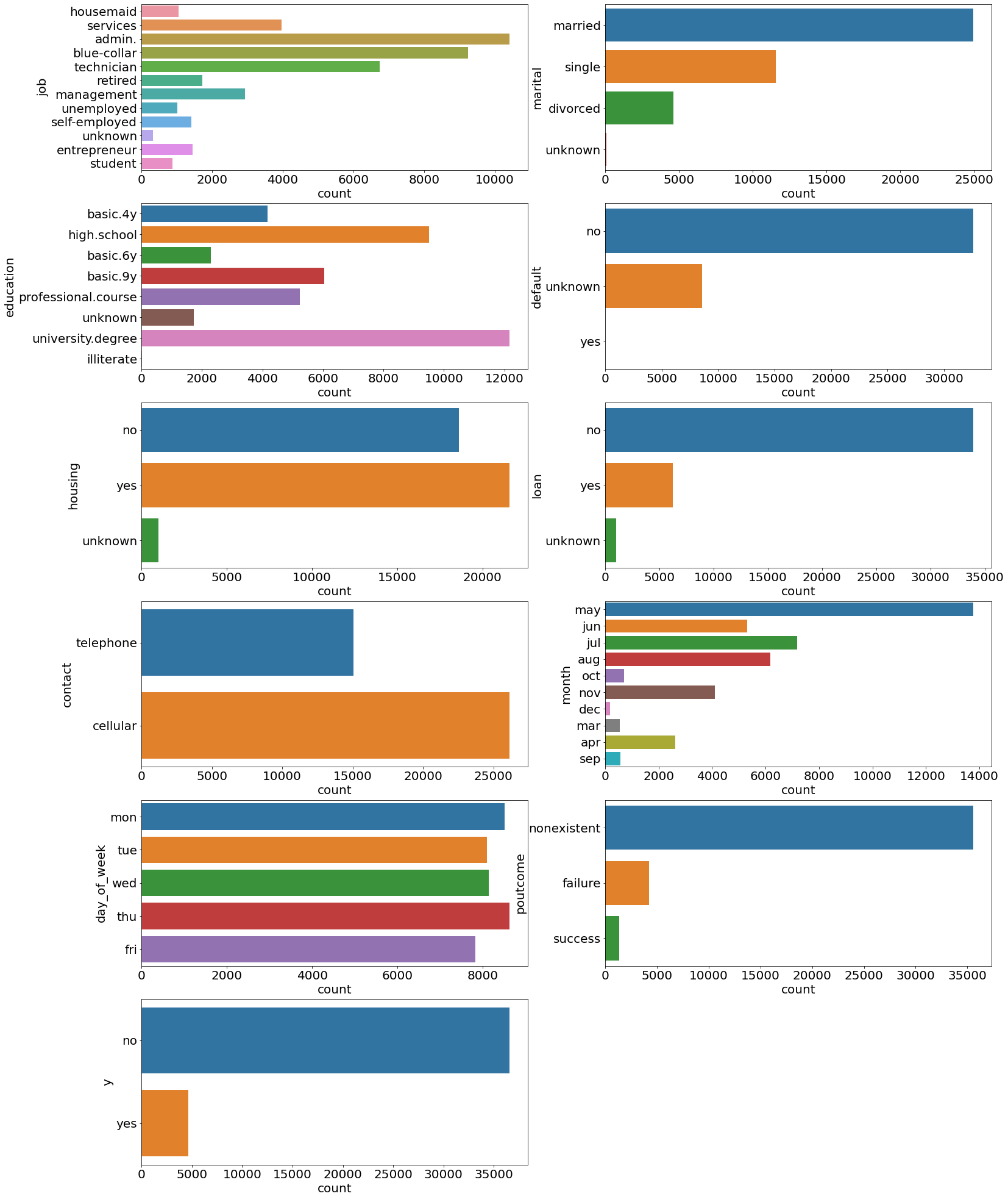
Initial data analysis

Loading the data and performing some initial exploration on it to acquire some basic knowledge about the data, how the various features are distributed.

Importing libraries and packages

# Mathematical operations and data manipulation
import numpy as np
import pandas as pd

# Plotting
import seaborn as sns
import matplotlib.pyplot as plt

# Warnings
import warnings

warnings.filterwarnings("ignore")

%matplotlib inline

Set paths

# Path to datasets directory
data_path = "./datasets"
# Path to assets directory (for saving results to)
assets_path = "./assets"

Loading dataset

# load data
dataset = pd.read_csv(f"{data_path}/bank-additional-full.csv", sep=";")
dataset.head().T

	0	1	2	3	4
age	56	57	37	40	56
job	housemaid	services	services	admin.	services
marital	married	married	married	married	married
education	basic.4y	high.school	high.school	basic.6y	high.school
default	no	unknown	no	no	no
housing	no	no	yes	no	no
loan	no	no	no	no	yes
contact	telephone	telephone	telephone	telephone	telephone
month	may	may	may	may	may
day_of_week	mon	mon	mon	mon	mon
duration	261	149	226	151	307
campaign	1	1	1	1	1
pdays	999	999	999	999	999
previous	0	0	0	0	0
poutcome	nonexistent	nonexistent	nonexistent	nonexistent	nonexistent
emp.var.rate	1.1	1.1	1.1	1.1	1.1
cons.price.idx	93.994	93.994	93.994	93.994	93.994
cons.conf.idx	-36.4	-36.4	-36.4	-36.4	-36.4
euribor3m	4.857	4.857	4.857	4.857	4.857
nr.employed	5191.0	5191.0	5191.0	5191.0	5191.0
y	no	no	no	no	no

Exploring dataset

# Printing dimensionality of the data, columns, types and missing values
print(f"Data dimension: {dataset.shape}")
for col in dataset.columns:
    print(
        f"Column: {col:35} | "
        f"type: {str(dataset[col].dtype):7} | "
        f"missing values: {dataset[col].isna().sum():3d}"
    )

Data dimension: (41188, 21)
Column: age                                 | type: int64   | missing values:   0
Column: job                                 | type: object  | missing values:   0
Column: marital                             | type: object  | missing values:   0
Column: education                           | type: object  | missing values:   0
Column: default                             | type: object  | missing values:   0
Column: housing                             | type: object  | missing values:   0
Column: loan                                | type: object  | missing values:   0
Column: contact                             | type: object  | missing values:   0
Column: month                               | type: object  | missing values:   0
Column: day_of_week                         | type: object  | missing values:   0
Column: duration                            | type: int64   | missing values:   0
Column: campaign                            | type: int64   | missing values:   0
Column: pdays                               | type: int64   | missing values:   0
Column: previous                            | type: int64   | missing values:   0
Column: poutcome                            | type: object  | missing values:   0
Column: emp.var.rate                        | type: float64 | missing values:   0
Column: cons.price.idx                      | type: float64 | missing values:   0
Column: cons.conf.idx                       | type: float64 | missing values:   0
Column: euribor3m                           | type: float64 | missing values:   0
Column: nr.employed                         | type: float64 | missing values:   0
Column: y                                   | type: object  | missing values:   0

# Numerical features
numerical_features = [
    col
    for col in dataset.columns
    if np.issubdtype(dataset[col].dtype, np.number)
]
print(numerical_features)

['age', 'duration', 'campaign', 'pdays', 'previous', 'emp.var.rate', 'cons.price.idx', 'cons.conf.idx', 'euribor3m', 'nr.employed']

# Computing statistics on numerical features
dataset[numerical_features].describe().T

	count	mean	std	min	25%	50%	75%	max
age	41188.0	40.024060	10.421250	17.000	32.000	38.000	47.000	98.000
duration	41188.0	258.285010	259.279249	0.000	102.000	180.000	319.000	4918.000
campaign	41188.0	2.567593	2.770014	1.000	1.000	2.000	3.000	56.000
pdays	41188.0	962.475454	186.910907	0.000	999.000	999.000	999.000	999.000
previous	41188.0	0.172963	0.494901	0.000	0.000	0.000	0.000	7.000
emp.var.rate	41188.0	0.081886	1.570960	-3.400	-1.800	1.100	1.400	1.400
cons.price.idx	41188.0	93.575664	0.578840	92.201	93.075	93.749	93.994	94.767
cons.conf.idx	41188.0	-40.502600	4.628198	-50.800	-42.700	-41.800	-36.400	-26.900
euribor3m	41188.0	3.621291	1.734447	0.634	1.344	4.857	4.961	5.045
nr.employed	41188.0	5167.035911	72.251528	4963.600	5099.100	5191.000	5228.100	5228.100

# Distributions of numerical features
plt.figure(figsize=(10, 18))
for index, col in enumerate(numerical_features):
    plt.subplot(5, 2, index + 1)
    sns.distplot(dataset[col])
plt.savefig(
    f"{assets_path}/numerical_distributions.png", format="png", dpi=500
)

# Categorical features
categorical_features = [
    col
    for col in dataset.columns
    if pd.api.types.is_string_dtype(dataset[col])
]

# Distributions of categorical features
plt.figure(figsize=(25, 35))
for index, col in enumerate(categorical_features):
    plt.subplot(6, 2, index + 1)
    ax = sns.countplot(y=col, data=dataset)
    ax.set_xlabel("count", fontsize=20)
    ax.set_ylabel(col, fontsize=20)
    ax.tick_params(labelsize=20)

plt.savefig(f"{assets_path}/categorical_counts.png", format="png", dpi=500)

# Number of entries in y column
print("Total number of entries:")
print(dataset["y"].value_counts(ascending=True))
print()
print("Percentages:")
print(dataset["y"].value_counts(normalize=True, ascending=True) * 100)

Total number of entries:
yes     4640
no     36548
Name: y, dtype: int64

Percentages:
yes    11.265417
no     88.734583
Name: y, dtype: float64