

Preprocessing#
Loading the data and performing some initial exploration on it to acquire some basic knowledge about the data, how the various features are distributed.
Importing libraries and packages#
 1# Mathematical operations and data manipulation
 2import pandas as pd
 3
 4# Statistics
 5from scipy.stats import ttest_ind
 6
 7# Plotting
 8import seaborn as sns
 9import matplotlib.pyplot as plt
10
11# Warnings
12import warnings
13
14warnings.filterwarnings("ignore")
15
16%matplotlib inline
Set paths#
1# Path to datasets directory
2data_path = "./datasets"
3# Path to assets directory (for saving results to)
4assets_path = "./assets"
Loading dataset#
1# load data
2dataset = pd.read_csv(f"{data_path}/preprocessed_absenteism.csv")
3dataset.head()
| ID | Reason for absence | Month of absence | Day of the week | Seasons | Transportation expense | Distance from Residence to Work | Service time | Age | Work load Average/day | ... | Disciplinary failure | Education | Son | Social drinker | Social smoker | Pet | Weight | Height | Body mass index | Absenteeism time in hours | |
|---|---|---|---|---|---|---|---|---|---|---|---|---|---|---|---|---|---|---|---|---|---|
| 0 | 11 | 26 | July | Tuesday | Spring | 289 | 36 | 13 | 33 | 239.554 | ... | No | high_school | 2 | Yes | No | 1 | 90 | 172 | 30 | 4 |
| 1 | 36 | 0 | July | Tuesday | Spring | 118 | 13 | 18 | 50 | 239.554 | ... | Yes | high_school | 1 | Yes | No | 0 | 98 | 178 | 31 | 0 |
| 2 | 3 | 23 | July | Wednesday | Spring | 179 | 51 | 18 | 38 | 239.554 | ... | No | high_school | 0 | Yes | No | 0 | 89 | 170 | 31 | 2 |
| 3 | 7 | 7 | July | Thursday | Spring | 279 | 5 | 14 | 39 | 239.554 | ... | No | high_school | 2 | Yes | Yes | 0 | 68 | 168 | 24 | 4 |
| 4 | 11 | 23 | July | Thursday | Spring | 289 | 36 | 13 | 33 | 239.554 | ... | No | high_school | 2 | Yes | No | 1 | 90 | 172 | 30 | 2 |
5 rows × 21 columns
Exploring dataset#
1# Printing dimensionality of the data, columns, types and missing values
2print(f"Data dimension: {dataset.shape}")
3for col in dataset.columns:
4    print(
5        f"Column: {col:35} | "
6        f"type: {str(dataset[col].dtype):7} | "
7        f"missing values: {dataset[col].isna().sum():3d}"
8    )
Data dimension: (740, 21)
Column: ID                                  | type: int64   | missing values:   0
Column: Reason for absence                  | type: int64   | missing values:   0
Column: Month of absence                    | type: object  | missing values:   0
Column: Day of the week                     | type: object  | missing values:   0
Column: Seasons                             | type: object  | missing values:   0
Column: Transportation expense              | type: int64   | missing values:   0
Column: Distance from Residence to Work     | type: int64   | missing values:   0
Column: Service time                        | type: int64   | missing values:   0
Column: Age                                 | type: int64   | missing values:   0
Column: Work load Average/day               | type: float64 | missing values:   0
Column: Hit target                          | type: int64   | missing values:   0
Column: Disciplinary failure                | type: object  | missing values:   0
Column: Education                           | type: object  | missing values:   0
Column: Son                                 | type: int64   | missing values:   0
Column: Social drinker                      | type: object  | missing values:   0
Column: Social smoker                       | type: object  | missing values:   0
Column: Pet                                 | type: int64   | missing values:   0
Column: Weight                              | type: int64   | missing values:   0
Column: Height                              | type: int64   | missing values:   0
Column: Body mass index                     | type: int64   | missing values:   0
Column: Absenteeism time in hours           | type: int64   | missing values:   0
1# Computing statistics on numerical features
2dataset.describe().T
| count | mean | std | min | 25% | 50% | 75% | max | |
|---|---|---|---|---|---|---|---|---|
| ID | 740.0 | 18.017568 | 11.021247 | 1.000 | 9.000 | 18.000 | 28.000 | 36.000 |
| Reason for absence | 740.0 | 19.216216 | 8.433406 | 0.000 | 13.000 | 23.000 | 26.000 | 28.000 |
| Transportation expense | 740.0 | 221.329730 | 66.952223 | 118.000 | 179.000 | 225.000 | 260.000 | 388.000 |
| Distance from Residence to Work | 740.0 | 29.631081 | 14.836788 | 5.000 | 16.000 | 26.000 | 50.000 | 52.000 |
| Service time | 740.0 | 12.554054 | 4.384873 | 1.000 | 9.000 | 13.000 | 16.000 | 29.000 |
| Age | 740.0 | 36.450000 | 6.478772 | 27.000 | 31.000 | 37.000 | 40.000 | 58.000 |
| Work load Average/day | 740.0 | 271.490235 | 39.058116 | 205.917 | 244.387 | 264.249 | 294.217 | 378.884 |
| Hit target | 740.0 | 94.587838 | 3.779313 | 81.000 | 93.000 | 95.000 | 97.000 | 100.000 |
| Son | 740.0 | 1.018919 | 1.098489 | 0.000 | 0.000 | 1.000 | 2.000 | 4.000 |
| Pet | 740.0 | 0.745946 | 1.318258 | 0.000 | 0.000 | 0.000 | 1.000 | 8.000 |
| Weight | 740.0 | 79.035135 | 12.883211 | 56.000 | 69.000 | 83.000 | 89.000 | 108.000 |
| Height | 740.0 | 172.114865 | 6.034995 | 163.000 | 169.000 | 170.000 | 172.000 | 196.000 |
| Body mass index | 740.0 | 26.677027 | 4.285452 | 19.000 | 24.000 | 25.000 | 31.000 | 38.000 |
| Absenteeism time in hours | 740.0 | 6.924324 | 13.330998 | 0.000 | 2.000 | 3.000 | 8.000 | 120.000 |
Individual identification (ID)
Reason for absence (ICD). Absences attested by the International Code of Diseases (ICD) stratified into 21 categories (I to XXI) as follows:
I Certain infectious and parasitic diseases II Neoplasms III Diseases of the blood and blood-forming organs and certain disorders involving the immune mechanism IV Endocrine, nutritional and metabolic diseases V Mental and behavioural disorders VI Diseases of the nervous system VII Diseases of the eye and adnexa VIII Diseases of the ear and mastoid process IX Diseases of the circulatory system X Diseases of the respiratory system XI Diseases of the digestive system XII Diseases of the skin and subcutaneous tissue XIII Diseases of the musculoskeletal system and connective tissue XIV Diseases of the genitourinary system XV Pregnancy, childbirth and the puerperium XVI Certain conditions originating in the perinatal period XVII Congenital malformations, deformations and chromosomal abnormalities XVIII Symptoms, signs and abnormal clinical and laboratory findings, not elsewhere classified XIX Injury, poisoning and certain other consequences of external causes XX External causes of morbidity and mortality XXI Factors influencing health status and contact with health services.
And 7 categories without (CID) 2. patient follow-up (22), 3. medical consultation (23), 4. blood donation (24), 5. laboratory examination (25), 6. unjustified absence (26), 7. physiotherapy (27), 8. dental consultation (28).
Month of absence
Day of the week (Monday (2), Tuesday (3), Wednesday (4), Thursday (5), Friday (6))
Seasons (summer (1), autumn (2), winter (3), spring (4))
Transportation expense
Distance from Residence to Work (kilometers)
Service time
Age
Work load Average/day
Hit target
Disciplinary failure (yes=1; no=0)
Education (high school (1), graduate (2), postgraduate (3), master and doctor (4))
Son (number of children)
Social drinker (yes=1; no=0)
Social smoker (yes=1; no=0)
Pet (number of pet)
Weight
Height
Body mass index
Absenteeism time in hours (target)
Temporal plots#
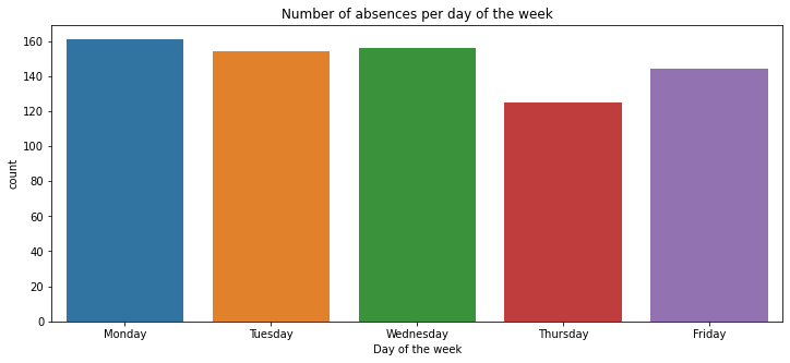
1# Counting entries per day of the week and month
2plt.figure(figsize=(12, 5))
3ax = sns.countplot(
4 data=dataset,
5 x="Day of the week",
6 order=["Monday", "Tuesday", "Wednesday", "Thursday", "Friday"],
7)
8ax.set_title("Number of absences per day of the week")
9plt.savefig(f"{assets_path}/dow_counts.png", format="png", dpi=300)
10
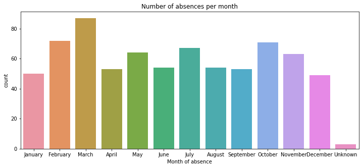
11plt.figure(figsize=(12, 5))
12ax = sns.countplot(
13 data=dataset,
14 x="Month of absence",
15 order=[
16 "January",
17 "February",
18 "March",
19 "April",
20 "May",
21 "June",
22 "July",
23 "August",
24 "September",
25 "October",
26 "November",
27 "December",
28 "Unknown",
29 ],
30)
31ax.set_title("Number of absences per month")
32plt.savefig(f"{assets_path}/month_counts.png", format="png", dpi=300)
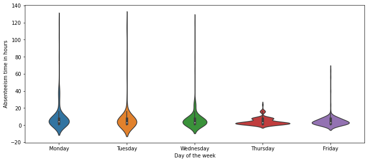
1# Analyse average distribution of absence hours
2plt.figure(figsize=(12, 5))
3sns.violinplot(
4 x="Day of the week",
5 y="Absenteeism time in hours",
6 data=dataset,
7 order=["Monday", "Tuesday", "Wednesday", "Thursday", "Friday"],
8)
9plt.savefig(f"{assets_path}/violin_dow_hours.png", format="png", dpi=300)
10
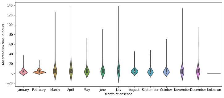
11plt.figure(figsize=(12, 5))
12sns.violinplot(
13 x="Month of absence",
14 y="Absenteeism time in hours",
15 data=dataset,
16 order=[
17 "January",
18 "February",
19 "March",
20 "April",
21 "May",
22 "June",
23 "July",
24 "August",
25 "September",
26 "October",
27 "November",
28 "December",
29 "Unknown",
30 ],
31)
32plt.savefig(f"{assets_path}/violin_month_hours.png", format="png", dpi=300)
 1# Computing mean and standard deviation of absence hours per day of
 2# the week
 3dows = ["Monday", "Tuesday", "Wednesday", "Thursday", "Friday"]
 4for dow in dows:
 5    mask = dataset["Day of the week"] == dow
 6    hours = dataset["Absenteeism time in hours"][mask]
 7    mean = hours.mean()
 8    stddev = hours.std()
 9    print(
10        f"Day of the week: {dow:10s} | Mean : {mean:.03f} | "
11        f"Stddev: {stddev:.03f}"
12    )
Day of the week: Monday     | Mean : 9.248 | Stddev: 15.973
Day of the week: Tuesday    | Mean : 7.981 | Stddev: 18.027
Day of the week: Wednesday  | Mean : 7.147 | Stddev: 13.268
Day of the week: Thursday   | Mean : 4.424 | Stddev: 4.266
Day of the week: Friday     | Mean : 5.125 | Stddev: 7.911
 1# Computing mean and standard deviation of absence hours per day of the month
 2months = [
 3    "January",
 4    "February",
 5    "March",
 6    "April",
 7    "May",
 8    "June",
 9    "July",
10    "August",
11    "September",
12    "October",
13    "November",
14    "December",
15]
16for month in months:
17    mask = dataset["Month of absence"] == month
18    hours = dataset["Absenteeism time in hours"][mask]
19    mean = hours.mean()
20    stddev = hours.std()
21    print(f"Month: {month:10s} | Mean : {mean:8.03f} | Stddev: {stddev:8.03f}")
Month: January    | Mean :    4.440 | Stddev:    5.786
Month: February   | Mean :    4.083 | Stddev:    3.710
Month: March      | Mean :    8.793 | Stddev:   16.893
Month: April      | Mean :    9.094 | Stddev:   18.024
Month: May        | Mean :    6.250 | Stddev:   10.314
Month: June       | Mean :    7.611 | Stddev:   12.359
Month: July       | Mean :   10.955 | Stddev:   21.547
Month: August     | Mean :    5.333 | Stddev:    5.749
Month: September  | Mean :    5.509 | Stddev:    8.407
Month: October    | Mean :    4.915 | Stddev:    8.055
Month: November   | Mean :    7.508 | Stddev:   16.121
Month: December   | Mean :    8.449 | Stddev:   16.049
 1# Statistical test for avg duration difference
 2thursday_mask = dataset["Day of the week"] == "Thursday"
 3july_mask = dataset["Month of absence"] == "July"
 4
 5thursday_data = dataset["Absenteeism time in hours"][thursday_mask]
 6no_thursday_data = dataset["Absenteeism time in hours"][~thursday_mask]
 7july_data = dataset["Absenteeism time in hours"][july_mask]
 8no_july_data = dataset["Absenteeism time in hours"][~july_mask]
 9
10thursday_res = ttest_ind(thursday_data, no_thursday_data)
11july_res = ttest_ind(july_data, no_july_data)
12
13print(
14    f"Thursday test result: statistic={thursday_res[0]:.3f}, "
15    f"pvalue={thursday_res[1]:.3f}"
16)
17print(
18    f"July test result: statistic={july_res[0]:.3f}, "
19    f"pvalue={july_res[1]:.3f}"
20)
Thursday test result: statistic=-2.307, pvalue=0.021
July test result: statistic=2.605, pvalue=0.009